# Initialize Otter
import otter
grader = otter.Notebook("game-theory.ipynb") | Economic Models, Fall 2024 |
Game Theory and Behavioral Economics
In this notebook, we will introduce a fundamental thought experiment in the economics and statistics subdomain of game theory, called the Prisoner’s Dilemma. We will then extend our consideration of game theory and behavioral economics to look at a recent paper that explores a phenomenon at the intersection of these topics.
At the end of this project, you should:
Understand the prisoner’s dilemma and strategies for playing the game
Understand the game theory underpinnings of the Thomas and Pemstein (2015) paper
Be able to rerun the analysis in the aforementioned paper using hypothesis testing
from datascience import *
import numpy as np, pandas as pd, datetime as dt
import seaborn as sns, matplotlib.pyplot as plt

%matplotlib inline
plt.style.use('seaborn-v0_8-muted')
plt.rcParams['figure.figsize'] = [25,10]

import warnings
warnings.simplefilter('ignore')

import httpimport
with httpimport.remote_repo("https://cal-icor.github.io/textbook.data/ucb/data-88e/"):
    from players import *
Part 1: The Iterated Prisoner’s Dilemma
The prisoner’s dilemma is a classic game first discussed by Merrill Flood and Melvin Dresher in 1950. In this game, there are two prisoners who have been captured and are being interrogated. The prisoners cannot contact each other in any way. They have two options: they can defect (betray the other prisoner to the police) or they can cooperate (maintain their silence). If both defect, both receive 4 years in prison. If one defects and the other does not, the defector goes free and the cooperator receives 5 years in prison. If both cooperate (meaning neither talks to the police), then they each receive 2 years in prison. We define mutual defection as the case when both prisoners defect and mutual cooperation as the case when both cooperate. The purpose of this game is to consider how a completely rational person would be best advised to proceed, and how different strategies for playing this game can be more or less effective.
| Prisoner A | |||
| Cooperate | Defect | ||
| Prisoner B | Cooperate | A: 2, B: 2 | A: 0, B: 5 |
| Defect | A: 5, B: 0 | A: 4, B: 4 | |
In this project, we will study the iterated prisoner’s dilemma, a game paradigm in which the prisoner’s dilemma is played over multiple rounds and in tournaments to determine the best strategy for playing the game. In this way, we define strategies as methods for determining whether a play will cooperate or defect at any single round based on this history of past moves. This differs from the normal prisoner’s dilemma in that we play the game multiple times and incorporate strategies going beyond any single iteration.
This paradigm was introduced by Robert Axelrod to use the prisoner’s dilemma as a lens through which to study the Cold War during the Cuban Missile Crisis. Axelrod created a tournament out of an iterated prisoner’s dilemma and invited theoreticians to write programs that could strategically play the game, and then pitted them one against another in a round-robin-style tournament.
Question 1.1: In the context of price wars, which prisoner’s dilemma outcome is best for consumers? Why?
Type your answer here, replacing this text.
In this project, we will be creating some custom Python classes to represent different playing strategies. We’ll be using the create_player_class function (provided) to create these classes for us. Here are a few important things to know about the classes:
Consider a player class instance player = Player().
player.play()is a method that represents a single move. It returnsTrueif the player defects andFalseif they cooperate.player.historyis an array of the previous moves of the player instance.player.history.item(-1), for example, is the most recent move (the last element of the array).
Don’t worry about the other methods that are defined for players; these are there for the code below to work but you don’t need to concern yourself with them. Here’s how the create_player_class function works:
Define a function,
f, that takes two arguments:selfandopponent(more about these later), and returnsTrueif the player defects andFalseotherwise.Call
create_player_classwith two arguments: a string for the class name, e.g."Player", and the play methodf.
Let’s illustrate this by creating Defector, a player that always defects. The defector_play function below always returns True, since the player always defects. We then create Defector using create_player_class.
def defector_play(self, opponent):
    return True

Defector = create_player_class("Defector", defector_play)
Just like any class, we create a Defector instance by calling the constructor:
Defector()Question 1.2: Create a Cooperator class that always cooperates.
def cooperator_play(self, opponent):
    return ...

Cooperator = ...grader.check("q1_2")Now that we have players, how do we pit them against each other? Provided is a function called payoff that returns the values from our payoff matrix when provided two players by using their play methods. payoff returns a tuple of 2 elements corresponding to the payoff for the first and second player:
>>> payoff(player_1, player_2)
(player 1 payoff, player 2 payoff)
payoff(Defector(), Cooperator())Our analysis of the prisoner’s dilemma hinges on analyzing strategies over multiple rounds. For this reason, we need a way to pit players against each other and find out who has the fewest years accrued. The function run_match below will run a match of two players with n turns. If winner is True, it returns the winner of the match; if winner is False, it returns a list for each player containing the sequence of years accrued. Also note the first two lines of the function that reset the player history for each player. This is important because we might end up reusing instances of players, and we don’t want histories from past matches to affect the results of this match.
def run_match(p1, p2, n=5, winner=True):
    p1.reset_history()
    p2.reset_history()

    p1_years = make_array()
    p2_years = make_array()

    for i in range(n):
        p1_score, p2_score = payoff(p1, p2)
        p1_years = np.append(p1_years, p1_score)
        p2_years = np.append(p2_years, p2_score)

    if winner:
        p1_mean = np.mean(p1_years)
        p2_mean = np.mean(p2_years)

        if p1_mean < p2_mean:
            return p1
        else:
            return p2
    else:
        return p1_years, p2_years
For example, we can run a 10-turn match between a defector and cooperator with:
run_match(Defector(), Cooperator(), n=10)We see that the defector won the match, as expected. We can get the raw data (the number of years accrued by each player at each iteration) by setting winner=False:
run_match(Defector(), Cooperator(), n=10, winner=False)Now that we know how to run matches, let’s think of some other cool strategies. Remember the player.history variable discussed earlier? Let’s have a concrete example on how to use that. The Alternator player defined below alternates between cooperating and defecting, beginning with cooperating.
Note the if statement. We need to check that we have a history to index into before we try to grab the last element; if we didn’t have that statement, the code would fail on the first time Alternator played, because we would try to get an element from an array with 0 elements.
def alternator_play(self, opponent):
    if len(self.history) > 0:
        return not self.history.item(-1)
    else:
        return False

Alternator = create_player_class("Alternator", alternator_play)

run_match(Alternator(), Defector())
Question 1.3: Use the player history to define TitForTat, a player that does the last thing it’s opponent did and starts off by cooperating. For example, if we pitted TitForTat against a Defector in a 5-round match, the Defector’s moves would be [D, D, D, D, D], and TitForTat’s would be [C, D, D, D, D].
def tit_for_tat_play(self, opponent):
    if len(opponent.history) > 0:
        return ...
    else:
        return ...

TitForTat = ...grader.check("q1_3")Now that we can pit two players against each other, how do we compare multiple players? We can create a tournament that runs matches between each pair of players.
Question 1.4: In a tournament with players, how many matches are run?
Hint: At an iteration , how many players does player play against? Do you repeat any matches?
Type your answer here, replacing this text.
To run through the tournament, we’ll need to iterate through each player and pit them against every other player in a match. To ensure that we don’t duplicate matches, we’ll loop from 0 to the number of players in the outer loop and loop from the next player to the last player in the inner loop. The function most_common returns the value in an array of values that has the largest number of occurrences; it is here used to determine which player won the most times.
players = make_array(Defector(), Cooperator())
winners = make_array()
for i in range(len(players)):
    for j in range(i+1, len(players)):
        winner = run_match(players.item(i), players.item(j))
        winners = np.append(winners, winner)

biggest_winner = most_common(winners)
biggest_winner
Question 1.5: Consider the four strategies we’ve defined so far: defector, cooperator, alternator, and tit-for-tat. Which strategy do you think would win in a tournament between these four? Why?
Type your answer here, replacing this text.
All of the strategies described in the table below, excepted TitForTat and ForgivingTitForTat, are provided.
| Name | Description |
|---|---|
Alternator | Alternates between C and D |
Backstabber | Forgives first 3 opponent D’s then D forever after fourth |
Bully | Starts by defecting and then does the opposite of opponent’s previous move |
Desperate | Only cooperates after mutual defection |
FoolMeOnce | Forgives one D then retaliates forever on a second D |
Forgiver | Starts by cooperating however will defect if at any point the opponent has defected more than 10 percent of the time |
ForgivingTitForTat | Starts by cooperating and defects if opponent has defected more than 10% of the time and their last move was defection |
Grudger | Starts with C and then D forever on opponent’s first D |
OnceBitten | C once on opponent D, but if opponent D’s twice in a row defaults to D for 10 turns |
TitForTat | Repeats opponent’s previous move |
Question 1.6: Suppose we have a 10-turn match with a backstabber and a desperate. Write down the sequence of defections (D) and cooperations (C) for each player. Who wins the match?
backstabber_moves = make_array(...)
desperate_moves = make_array(...)
backstabber_desperate_winner = "..."grader.check("q1_6")Question 1.7: Implement the player ForgivingTitForTat as described in the table above. The percentage should be calculated at each turn, so that if the opponent defects to above 10% and then lowers their defection percentage below 10% the ForgivingTitForTat player should cooperate.
Hint: You can get the number of defections in a player’s history by summing it or using np.count_nonzero, as defections are recorded as True.
def forgiving_tit_for_tat_play(self, opponent):
    if len(self.history) == 0:
        return ...
    return ... and ...

ForgivingTitForTat = create_player_class("ForgivingTitForTat", forgiving_tit_for_tat_play)grader.check("q1_7")Tournaments
Now that we have re-familiarized ourselves with our prisoner’s dilemma code from the lab, let’s move on to recreating Axelrod’s tournament. Recall that Axelrod originally wanted to compare strategies for playing the prisoner’s dilemma, which he did by pitting every strategy against every other strategy in a round-robin tournament. In this project, we will do the same thing, albeit on a much smaller scale, with the strategies defined in the table above.
Question 1.8: Fill in the function run_tournament below that takes in an array of players and returns a table with four columns: p1, p1_mean, p2, and p2_mean. As in Axelrod’s original tournament, use matches with 200 rounds.
Hint: Recall how we can use the winner argument of run_match.
def run_tournament(players):
    p1 = make_array() #This stores an array of all player 1's.
    p2 = make_array() #This stores an array of all player 2's.
    p1_means = make_array() #This stores an array of each player 1's average jail time for a particular game.
    p2_means = make_array() #This stores an array of each player 2's average jail time for a particular game.

    for i in range(len(players)):
        for j in range(i+1, len(players)):
            p1_years, p2_years = run_match(..., ..., n=200, winner=...)
            p1 = np.append(..., players.item(...))
            p2 = np.append(..., players.item(...))
            p1_means = np.append(..., ...(p1_years))
            p2_means = np.append(..., ...(p2_years))

    results = Table().with_columns(
        "p1", p1,
        "p1_mean", p1_means,
        "p2", p2,
        "p2_mean", p2_means
    )

    return results

run_tournament(make_array(Defector(), Cooperator()))grader.check("q1_8")Question 1.9: Create a tournament with all players in the table above Question 1.6. Assign the results table to tournament_results.
all_strategies = make_array(...)
tournament_results = run_tournament(...)
tournament_resultsgrader.check("q1_9")To visualize our results, we will make a heat map that displays our results in an easy-to-read manner. The code in the cell below uses seaborn and pandas, two libraries you will learn about in Data 100, so don’t worry about understanding it.
The plot shows Player 1 on the horizontal axis, Player 2 on the vertical axis, and the values in the cells are Player 1’s mean score (i.e. the mean score of the player on the horizontal axis). So, if we look at the intersection of OnceBitten on the horizontal and Forgiver on the vertical, we see OnceBitten’s mean of 2.000 and if we do the reverse (Forgiver on horizontal, OnceBitten on vertical), we see Forigiver’s mean of 2.000.
df1 = tournament_results.to_df()
df2 = tournament_results.to_df()
df2 = df2.rename({"p1": "p2", "p2": "p1", "p1_mean": "p2_mean", "p2_mean": "p1_mean"}, axis=1)
df = pd.concat([df1, df2])
df["p1"], df["p2"] = df["p1"].astype(str), df["p2"].astype(str)
df = df.pivot(index="p1", columns="p2", values="p1_mean")

plt.figure(figsize=[15,8])
sns.heatmap(df.T, annot=True, fmt=".3f")
plt.xlabel("Player 1")
plt.ylabel("Player 2")
plt.title("Player 1's Mean Scores by Opponent")
plt.xticks(rotation=90);
Question 1.10: Interpret the plot above. What results stand out to you? Which strategy would you choose if you were playing in a tournament? Justify your answer.
Type your answer here, replacing this text.
Now that we have the experience of creating prisoner’s dilemma tournaments, let’s consider Axelrod’s findings. The winning deterministic strategy was, surprisingly, tit-for-tat. This strategy was entered into the competition by Anatol Rapoport, coded in only four lines of BASIC. Axelrod studied the best strategies and came up with the following four traits of the biggest winners: niceness, retaliation, forgiveness, and lack of envy.
Question 1.11: In analyzing his tournament, Axelrod noted that one of the traits of the best strategies was being “non-envious.” A strategy that is non-envious does not strive to score higher than its opponent. Why do you think this trait is linked to good strategies? How does one of the other strategies you looked at (excluding defector, cooperator, and tit-for-tat) embody this trait?
Type your answer here, replacing this text.
Question 1.12: The prisoner’s dilemma is often used by economists to study and understand different phenomena that are observed in economies at different scales (e.g. studying oligopolies). Another common economic application is studying advertising and how the advertising of other firms needs to be taken into account in a single firm’s advertising strategies. Describe how firms in an advertising space can be viewed as players in an iterated prisoner’s dilemma. What decisions are analogous to defection and cooperation? What are the payoffs of each?
Type your answer here, replacing this text.
If you want to learn more about this tournament, there’s a very interesting episode of Radiolab that describes the origins of Axelrod’s tournament, the iterated prisoner’s dilemma, and the tit-for-tat strategy.
Part 2: Height Perceptions
For the rest of this project, we are going to move on to replicating the analysis in this paper by Thomas and Pemstein (2015). The paper describes two experiments, both of which we will cover in this project. Before doing this part, you may want to refresh your memory on A/B testing and p-values by rereading Chapters 11 and 12 of the Data 8 Textbook.
Take a moment to read the Experiment 1 methodology from the paper. Ensure you understand the experiment before moving on.
Question 2.1: The first experiment examined subjects’ perception of height by adjusting the
screen position
camera position
camera focus
camera exposure
Assign the letter corresponding to your answer to q2_1 below.
q2_1 = ...grader.check("q2_1")Now we’ll read in the experimental data from the paper. The table below gives the condition, height estimate, and true height for each subject. Recall that individuals can be in one of two conditions: “down”, where they’re looking up at the pictured individual, and “up”, where they’re looking down at the pictured individual.
exp1_raw = Table.read_table("https://cal-icor.github.io/textbook.data/ucb/data-88e/frontiers1.csv")
exp1_raw
In this section, we will be conducting an A/B test, wherein we split some data into two groups randomly and calculate some test statistic on each group. The first component of an A/B test is a test statistic, a value that we calculate that compares two groups. A good test statistic is one for which large or small values but not both indicate in the direction of the alternative hypothesis.
As a precursor to our test statistic (i.e. not as the test statistic itself), we will calculate the error ratio between the estimate and the true height:
This will give us the magnitude of the difference relative to the true height, to correct for any scale differences based on the actual height of the figure, and whether the estimate was above or below the actual height.
Question 2.2: How can we turn the error ratio column into a good test statistic for comparing the two conditions?
take the signed difference of the standard deviation of the error ratios for both groups
take the absolute difference of the standard deviation of the error ratios for both groups
take the signed difference of the mean error ratios for both groups
take the absolute difference of the mean error ratios for both groups
Assign the letter corresponding to your answer to q2_1 below.
q2_2 = ...grader.check("q2_2")Question 2.3: Add an ErrorRatio column to exp1_raw with the error ratio using the formula above. Store the resulting table as exp1.
error_ratio = ...
exp1 = ...
exp1grader.check("q2_3")Now that we have quantified the error of each estimate, let’s take a look at the distributions of these values in order to develop some intuition before we generate our alternative hypothesis.
Question 2.4: Plot overlaid histograms of the ErrorRatio column grouped by Condition.
Hint: Recall that we can created a grouped histogram of a column of a table using tbl.hist(..., group=GROUP_COLUMN).
...Question 2.5: Interpret the histogram you just created. What can you say about the distributions of the up- and down-conditions?
Hint: Look at where each histogram is centered.
Type your answer here, replacing this text.
Now that we know how we can quantify the difference between the estimate and true height and we have some idea of their distributions, how can we determine if the differences between the two are drawn from different distributions based on the condition?
Question 2.6: What are the null and alternative hypotheses for our A/B test?
Null hypothesis: Type your answer here, replacing this text.
Alternative hypothesis: Type your answer here, replacing this text.
Before we get into performing the A/B test, we need to create a way for us to easily calculate the error ratios for each iteration.
Question 2.7: Fill in the function add_error_ratio which will take in a table, create the ErrorRatio column as above, and return a new table.
def add_error_ratio(tbl):
    """Adds error ratio column to tbl"""
    error_ratio = ...
    tbl = ...
return tblgrader.check("q2_7")In order to run an A/B test, we need to choose a test statistic. Recall that a good test statistic indicates in the direction of the alternative hypothesis at very high or very low values. In this case, we will use the mean error ratio for each group, which indicates the alternative at higher values.
The function calc_abs_diff_mean_error_ratio defined below will calculate the error ratios, compute the mean for each group, and return the absolute difference between the two. Note that it requires your add_error_ratio function to work correctly.
def calc_abs_diff_mean_error_ratio(tbl):
    """Calculates absolute difference between mean error ratios"""
    tbl = add_error_ratio(tbl)
    grouped = tbl.group("Condition", np.mean)
    return abs(grouped.column("ErrorRatio mean").item(0) - grouped.column("ErrorRatio mean").item(1))
OK, now we have all the pieces we need to perform an A/B test. Recall that in the general outline of an A/B test, we
shuffle the condition we’re examining several times
calculate the test statistic on each of the shuffled conditions
collect these statistic values somewhere
compute the observed value of the test statistic (i.e. the test statistic on the original data)
compute the p-value as the proportion of values further in the direction of the alternative hypothesis than the observed value
An outline for the code of this process might be:
test_statistics = make_array()
for i in range(n):
    shuffled_conditions = # shuffle the table and grab conditions
    shuffled_table = # replace condition column with shuffled_conditions
    test_statistic = # value of test statistic on shuffled conditions
    test_statistics = # append test_statistic to test_statistics

observed_value = # value of test statistic on original data
p_value = # proportion of test_statistics <=/>= observed_value
Question 2.8: In the cell below, fill in the code to run the A/B test on our data and collect the test statistic values in ratio_diffs. Recall that to run an A/B test we need to shuffle the values of the Condition column, drop the original column, and add in the new values.
ratio_diffs = make_array()

for i in np.arange(1000):
    conditions = ...
    shuffled_exp1 = ...
    ratio_diffs = ...

ratio_diffs[:5]grader.check("q2_8")To determine the results of our A/B test, we need to calculate a p-value. To calculate the p-value, we find the percentage of results wherein the test statistic was further in the direction of the alternative hypothesis than the observed value.
Question 2.9: Calculate the observed value of the test statistic using the calc_abs_diff_mean_error_ratio function and store it as observed_value. Then calculate the p-value and store it as p_value.
Hint: Do values above or below observed_value indicate the alternative hypothesis?
observed_value = ...
p_value = ...
p_valuegrader.check("q2_9")Question 2.10: Using the conventional p-value cutoff of 0.05, which hypothesis do we adopt?
null hypothesis
alternative hypothesis
q2_10 = ...grader.check("q2_10")Part 3: Height Perceptions and the Game
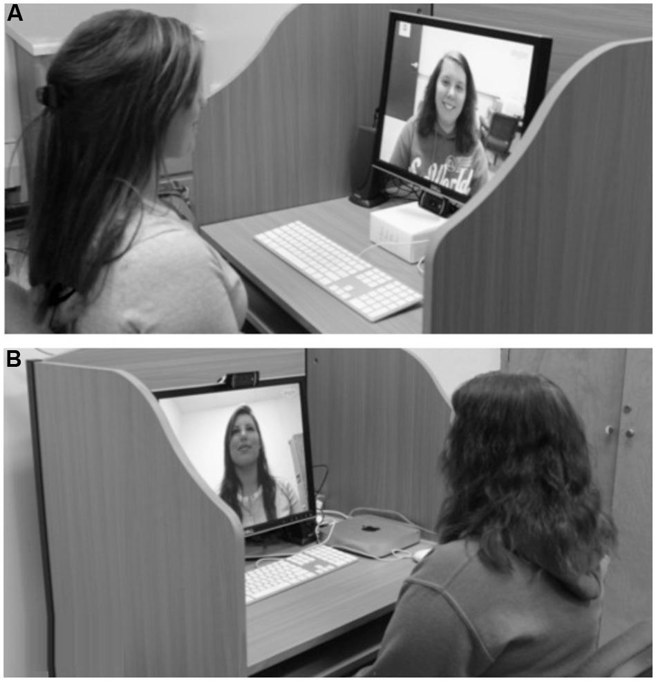
In this section of the project, we will look at the second experiment from Thomas and Pemstein (2015). In this experiment, the placement of cameras is used to determine what effect the perception of height has on the leader-follower behavior of subjects.
Take a moment to read the Experiment 2 methodology from the paper. Ensure you understand the experiment before moving on.
The payoff structure of the game is reproduced below for your reference.
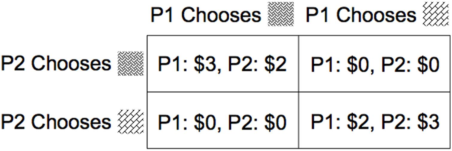
Note: In the rest of this project,  will be referred to as the “chainmail pattern” and
  as the “brick pattern.”
Question 3.1: If Player 1 chooses the chainmail pattern and Player 2 the brick pattern, what is the payoff for each player?
1: \$0, 2: \$2
1: \$2, 2: \$3
1: \$3, 2: \$2
1: \$0, 2: \$0
Assign the letter corresponding to your answer to q3_1 below.
q3_1 = ...grader.check("q3_1")Question 3.2: What is meant by the “asymmetrical condition” in the paper?
cameras are placed on different sides (left/right) of the monitor
one camera is up or down and the other is in the center of the monitor
one camera is up and the other is down
both cameras are on the same side of the monitor (both up or both down)
Assign the letter corresponding to your answer to q3_2 below.
q3_2 = ...grader.check("q3_2")Now we’ll read in the data from the experiment. The Condition column here indicates whether the subjects are in the asymmetrical (1) or symmetrical (2) condition. The Choice column indicates their choice of payoff (for themselves) and the Winnings column what they actually won.
exp2 = Table.read_table("https://cal-icor.github.io/textbook.data/ucb/data-88e/frontiers2.csv")
exp2
In order to determine whether the camera placement had an effect on the payoff choice in the experimental condition, we need to check that people in the one condition chose the payoff-maximizing choice more often that people in the other condition. Let’s start by limiting the data to subjects in the experimental condition and creating a variable that indicates whether the subject chose the payoff-maximizing value.
Question 3.3: Filter exp2 for rows in the experimental condition (Condition is 1) and store this as exp_condition. Then add a column to exp_condition that indicates whether the subject chose the payoff-maximizing value by applying the provided payoff_maximizing function to the Choice column; store this as the Payoff column.
def payoff_maximizing(val):
    return int(val == 3)

exp_condition = ...
payoffs = ...
exp_condition = ...
exp_conditiongrader.check("q3_3")Now that we know which subjects chose the payoff-maximizing value, we can run an A/B test on this variable to determine whether the Room variable (which indicates whether the camera was up or down) has any effect on the outcome. We’ll use the absolute difference between the proportion of 1’s in each group as our test statistic. The provided function payoff_proportion will calculate this value when provided an array of Payoff values.
def payoff_proportion(payoffs):
    return np.sum(payoffs) / len(payoffs)

payoff_proportion(make_array(0, 1, 0, 1))
Now that we know how to calculate the test statistic, let’s think about how we can group our table for the A/B test. We’ll need to group on the Room variable, and we can use our payoff_proportion function as the collection function for Table.group.
grouped_exp = exp_condition.group("Room", payoff_proportion)
grouped_exp
Now that we have the grouped values, we can calculate our test statistic by taking the absolute difference of the two values.
payoff_props = grouped_exp.column("Payoff payoff_proportion")
abs(payoff_props.item(0) - payoff_props.item(1))
With the logic for how we calculate the test statistic value in place, let’s write a function that will do this for us in each loop of the A/B test.
Question 3.4: Fill in the function calc_condition_test_stat below which runs through the logic above for a provided table tbl.
Hint: You can check that your function is correct by comparing the cell’s output to the last code cell.
def calc_condition_test_stat(tbl):
    grouped_exp = ...
    payoff_props = ...
    ...

calc_condition_test_stat(exp_condition)grader.check("q3_4")Now that we have an easy way to calculate the test statistic, let’s build our A/B test. Recall that we will need to shuffle the values of the Room variable and then run calc_condition_test_stat on the resulting table.
Question 3.5: Fill in the code below to run the A/B test and collect our test statistic values in condition_stat_values.
condition_stat_values = make_array()
for i in np.arange(1000):
    conditions = ...
    shuffled_exp_condition = ...
    stat_value = ...
    condition_stat_values = ...

condition_stat_values[0:5]grader.check("q3_5")Now let’s calculate our p-value. As with before, values higher than the observed value indicate the alternative hypothesis, so we’ll be looking for those again.
Question 3.6: Fill in the code below to store the observed value as condition_observed_value and the p-value as condition_p_value.
condition_observed_value = ...
condition_p_value = ...
condition_p_valuegrader.check("q3_6")Question 3.7: Using the conventional p-value cutoff of 0.05, which hypothesis do we adopt?
null hypothesis
alternative hypothesis
q3_7 = ...grader.check("q3_7")References
Thomas, L. E., & D. Pemstein (2015). “What you see is what you get: webcam placement influences perception and social coordination.” Frontiers in Psychology. Thomas & Pemstein (2015)
Submission
Make sure you have run all cells in your notebook in order before running the cell below, so that all images/graphs appear in the output. The cell below will generate a zip file for you to submit. Please save before exporting!
# Save your notebook first, then run this cell to export your submission.
grader.export(run_tests=True)- Thomas, L. E., & Pemstein, D. (2015). What you see is what you get: webcam placement influences perception and social coordination. Frontiers in Psychology, 6. 10.3389/fpsyg.2015.00306
- Thomas, L. E., & Pemstein, D. (2015). What you see is what you get: webcam placement influences perception and social coordination. Frontiers in Psychology, 6. 10.3389/fpsyg.2015.00306