# Initialize Otter
import otter
grader = otter.Notebook("econometrics.ipynb") | Economic Models, Fall 2024 |
Econometrics
In the textbook and this week’s lecture, we gave you a theoretical introduction to econometrics. In this project, you’ll get the chance to apply what you’ve learned and see how econometrics is actually used by economists!
This project is based on an influential study on the relationship between a person’s height and labor market outcomes, and is divided into 3 sections:
Simple Linear Regression
Multiple Linear Regression
Reading Econometrics Tables
You can refer to the Econometrics chapter in the textbook and week 11 resources for help on this project.
from datascience import *
import numpy as np
import pandas as pd
import statsmodels.api as sm
Part 1: Simple Linear Regression
Several studies have identified a positive correlation between a person’s height and labor market outcomes: on average, taller people have jobs that are of a higher status and pay more. In their paper, Stature and Status: Height, Ability, and Labor Market Outcomes (2008), economists Anne Case and Christina Paxson analyze the data from the US National Health Interview Survey in 1994 to explain this association. This is the data we will be using for our analysis.
In the first part of the project, we will use simple (bivariate) linear regression to look at the association between a person’s height and earnings, and consider the problems with limiting our regression model to just 1 regressor.
We start by importing the earnings.csv dataset which contains information about the characteristics and labor market outcomes for 17,870 workers.
earnings = Table().read_table("https://cal-icor.github.io/textbook.data/ucb/data-88e/earnings.csv")
earnings.show(5)
Before proceeding, please read the data description for this study which gives you information about each variable. This is very important.
Question 1.1: What do you expect the sign of the relationship between height and earnings to be? Explain your answer.
Type your answer here, replacing this text.
Note: We generally take the log of earnings in regression models but we’re not doing that in this project for the sake of simplicity. We’ll be using log earnings as the dependent variable in section 3.
Question 1.2: Here’s a simple linear regression equation to model the association between height and earnings:
Perform a regression of earnings on height. Don’t forget to add a constant term!
y_1_2 = ...
x_1_2 = ...
model_1_2 = ...
results_1_2 = ...
results_1_2.summary()grader.check("q1_2")Question 1.3: Why should we include a constant term in this regression model?
Because we expect the slope of the line of best fit may be zero.
Because we expect the slope of the line of best fit may be non-zero.
Because we expect the x-intercept of the line of best fit may be non-zero.
Because we expect the y-intercept of the line of best fit may be non-zero.
Assign a letter corresponding to your answer to q1_3 below. For example, q1_3 = 'a'.
q1_3 = ...grader.check("q1_3")Question 1.4: What is the estimated association between earnings and height?
result_1_4 = ...
result_1_4grader.check("q1_4")Question 1.5: Is the association statistically significant? Answer True or False.
result_1_5 = ...
result_1_5grader.check("q1_5")Question 1.6: Interpret the slope on the height variable (including the units).
A 1 inch increase in height corresponds to around a \$707.7 increase in earnings
A 1 inch increase in height corresponds to around a \$707.7 decrease in earnings
A 1% increase in height corresponds to around a \$707.7 increase in earnings
A 1% increase in height corresponds to around a \$707.7 decrease in earnings
Assign a letter corresponding to your answer to q1_6 below. For example, q1_6 = 'a'.
q1_6 = ...grader.check("q1_6")Question 1.7: Interpret the intercept of the regression (including the units). Does this make practical sense?
When height is 0, earnings are estimated to be around -\$512.7.
When height is 0, earnings are estimated to be around \$512.7.
When earnings are 0, height is estimated to be around -512.7 inches.
When earnings are 0, height is estimated to be around 512.7 inches.
Assign a letter corresponding to your answer to q1_7 below. For example, q1_7 = 'a'.
q1_7 = ...grader.check("q1_7")Question 1.8: If the slope on the independent variable is statistically significant, can we infer a causal relationship between the two variables? Why or why not? When can you infer a causal relationship between 2 variables based on the results of the study?
Hint: Think about the type of study we’re looking at.
Type your answer here, replacing this text.
Question 1.9: Use the slope and intercept from the regression in question 1.2 to generate predictions for earnings.
predictions_1_9 = ...
predictions_1_9grader.check("q1_9")Question 1.10: Calculate the RMSE for your regression predictions from question 1.9.
rmse_1_10 = ...
rmse_1_10grader.check("q1_10")Question 1.11: Which one of the following is true about the RMSE?
RMSE is the total sum of squared error in the regression.
RMSE means that on average the predicted earnings are off by $26,775.7.
It is possible for the RMSE to increase if we add unrelated variables to the regression.
Higher RMSE means the model more accurately predicts the dependent variable.
Assign a letter corresponding to your answer to q1_11 below. For example, q1_11 = 'a'.
q1_11 = ...grader.check("q1_11")Part 2: Multiple Linear Regression
Now, let’s perform multiple linear regression to account for potential confounding variables in our model. For simplicity, we will be using only the following additional regressors: age, educ, sex and weight.
Question 2.1: Pick 2 variables from the 4 additional variables we will be incorporating in the model (age, educ, sex and weight) that you think might be potential confounders in the study. Provide a brief explanation for why you think each of the variables may be a confounder.
Hint: Recall that a confounder is related to both the independent and dependent variables, so in your answer, make sure to talk about how each confounder is related to height and weight.
Type your answer here, replacing this text.
Question 2.2: Perform another regression with the following new regressors: age, educ, sex and weight (also include height).
y_2_2 = ...
x_2_2 = ...
model_2_2 = ...
results_2_2 = ...
results_2_2.summary()grader.check("q2_2")Question 2.3: Compare the coefficient on height from the regression model in question 2.2 to the coefficient on height from the regression model in question 1.2. What does this tell you about the nature of the omitted variable bias in the previous model (is it positive or negative)?
Fill in the blanks: The coefficient in 2.2 is _____ which means that the omitted variable bias in 1.2 is overall _____.
higher; positive
lower; positive
higher; negative
lower; negative
Assign a letter corresponding to your answer to q2_3 below. For example, q2_3 = 'a'.
q2_3 = ...grader.check("q2_3")Question 2.4: Look at the regression coefficients for the additional variables we included in question 2.2. Do the coefficients align with your intuition from 2.1 (in terms how they are related to earnings)?
Type your answer here, replacing this text.
Question 2.5: Let’s consider the effect of education on earnings. According to the result in 2.2, is the level of education correlated with earnings? Does adding this variable help alleviate omitted variable bias? Why or why not? Explain your answers.
Type your answer here, replacing this text.
Question 2.6: If we computed the RMSE for this new regression model, do you think it would be higher or lower than the RMSE we computed in 1.10?
Lower
Higher
It depends on the specific choice of variables
Assign a letter corresponding to your answer to q2_6 below. For example, q2_6 = 'a'.
q2_6 = ...grader.check("q2_6")Question 2.7: Now that we’ve accounted for some additional confounding variables do you think it makes sense for us to infer a causal relationship between height and earnings?
Yes, because the coefficient for height is now highly significant.
Yes, because we have eliminated omitted variable bias by adding control variables in 2.2.
No, because there may be other omitted variables we haven't accounted for.
No, because the set of control variables added in 2.2 is a poor choice.
Assign a letter corresponding to your answer to q2_7 below. For example, q2_7 = 'a'.
q2_7 = ...grader.check("q2_7")Question 2.8: Using regression results in 2.2, now let’s try to predict a person’s earnings based on their characteristics.
What would the predicted earnings of a 35-year-old woman with a Bachelor’s degree who is 64 inches tall and 124 pounds?
Hint: A person with a Bachelor’s degree has completed 15 years of education.
prediction_2_8 = ...
prediction_2_8grader.check("q2_8")Question 2.9: Say you wanted to know the relationship between gender (sex: a binary variable) and income (earnings: a continuous variable). Based on our regression results, how is gender correlated with income?
Hint: Think about what it means when the coefficient of sex is 0 and 1. Also, you can try changing your input for sex in 2.8, and see what happens.
Assuming all else equal, ...
On average, male earns \$586.92 more than female.
On average, female earns \$586.92 more than male.
For every 1 inch increase in height, male's income will increase on average \$586.92 more than that of female.
For every 1 inch increase in height, female's income will increase on average \$586.92 more than that of male.
Assign a letter corresponding to your answer to q2_9 below. For example, q2_9 = 'a'.
q2_9 = ...grader.check("q2_9")Part 3: Reading Econometrics Tables
Researchers tend to run multiple regression models which they summarize in econometrics tables.
Below is a table taken from the paper. It shows the regression results from 2 studies on the relationship between height and earnings: the British Cohort Study (BCS) and National Child Development Study (NCDS).
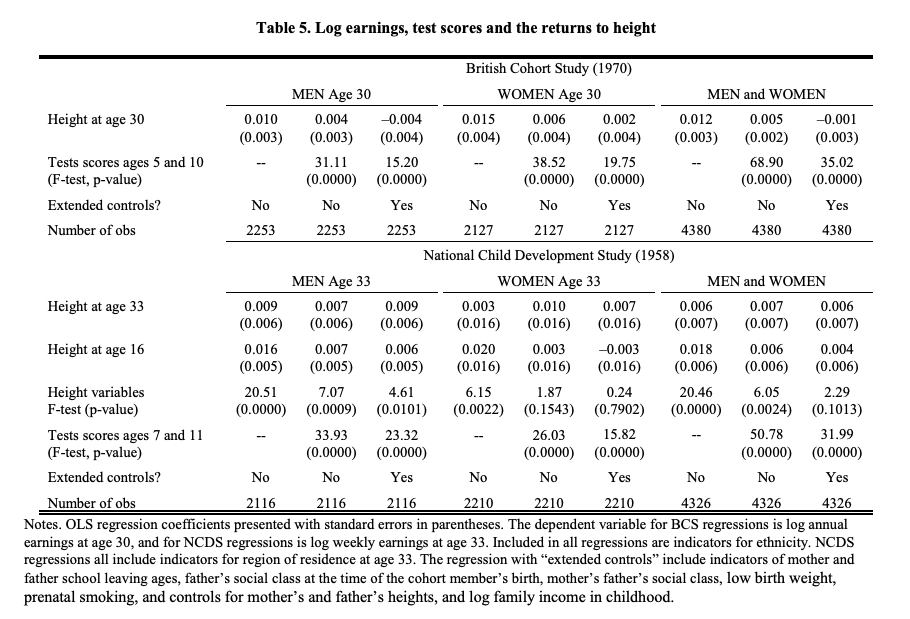
Make sure to read the table (including the note at the bottom) before proceeding.
Note that for the questions below, log earnings is the dependent variable. Recall the interpretation of the slope in this case.
Question 3.1: According to the table, what did the British Cohort Study (1970) find about the relationship between height at age 30, test scores ages 5 and 10, and earnings for women? Use the results with extended controls added in. Which of the followings are correct? There can be 1-4 correct answers.
The coefficient on height is statistically significant.
The coefficient on height means for every 1 inch increase in height at age 30, the annual earnings will on average increase by 0.002 dollars.
The coefficient on test scores is statistically significant.
The coefficient on test scores means for every 1 point increase in test scores ages 5 and 10, the annual earnings will on average increase by 19.75 dollars.
Assign an array of letters corresponding to your answer to q3_1 below. For example, q3_1 = make_array('a', 'b', 'c', 'd').
q3_1 = ...grader.check("q3_1")Question 3.2: Now look at the results of the British Cohort Study for men. There are 3 coefficients reported for height at age 30. Give a brief interpretation of each of these coefficients (including the units). In your explanation, talk about what is causing the differences among these coefficients (hint: look at the Test scores and Extended controls rows).
Note: Assume height is measured in inches for this study.
Type your answer here, replacing this text.
Conclusion
This brings us to the end of project 4! You’ve learned some key econometrics skills such as running regressions and reading econometrics tables. You’ve also developed an intuition for ordinary linear regression, omitted variable bias and regression with dummy variables.
Also, we didn’t cover a large part of Case and Paxson’s fascinating study so if you’re interested in how they explain the positive association between height and earnings, we recommend giving the paper a read!
Congratulations on finishing your final DATA 88E project! We’re so proud of you!
If you have any feedback for us, we’d love to hear it! Feel free to reach out to Akhil at akhil
Submission
Make sure you have run all cells in your notebook in order before running the cell below, so that all images/graphs appear in the output. The cell below will generate a zip file for you to submit. Please save before exporting!
# Save your notebook first, then run this cell to export your submission.
grader.export(run_tests=True)