Table of Contents
Oh Rats!: A Data Science Dive Into Invasive Species and Island Sustainability
Import Libraries and Their Aliases
Here we will import many of the industry-standard libraries including NumPy, Pandas, MatPlotLib, and Plotly. Feel free to find these packages on the Python Package Index!
For your reference, we’ll break down one line of the large cell below. In this line:
import pandas as pdWe import the pandas library. Essentially, we’re telling python that we want to use a specific set of functions that has been named “pandas”. We then use the as keyword to specify that we want to use some other name to refer to “pandas”; in this context we told python we want to call it “pd”.
Lets say we want to use the pandas.notnull() function (this checks if any values in an array or list are None).
Because we imported “pandas” as “pd”, we could now call pd.notnull()
Note: We name pandas as “pd” because it is the standard name in the industry, however we could have said:
import pandas as harrystylesWhich would’ve allowed us to run Harry_Styles.notnull(). This would be confusing for a reader, so its considered best practice to use standard names such as “pd” for “pandas” or “np” for “numpy”.
The cell below runs what we just talked about. Feel free to play around and try things out!
import pandas as pd
import pandas as harrystyles
print("Harry Styles is a Panda?", harrystyles == pd)
truth = [1, 2, 3, None, 4, harrystyles,
         "Harry Styles", None, None,
         5 * 2 - 1 / 1e-20, 1]
print(harrystyles.notnull(truth))
print(pd.notnull(truth))

# these lines delete the two imports we just made
del harrystyles
del pd
Now, lets get to work! Here we’ll import the actual modules we’ll need for this notebook!
#necessary to implement `download_data()` [see below]
import requests
from pathlib import Path
import time
#standard data analysis libraries
import numpy as np
import pandas as pd
#imports for displaying, rendering, and saving plots and visualizations
import plotly
import plotly.express as px
from IPython.display import *
import plotly.io as pio
import ipywidgets as widgets
from ipywidgets import *
#for dependency if not on datahub
# >>>%pip install openpyxl
Function Fun
download_data
The download_data function will get data from data_url on the Internet and saves it so we can use it for analysis!
This is a good practice to get into so that your future research or projects are reproducible. Essentially, if you gave someone else a copy of this notebook, they should be able to run all of the cells and get the same result. So, if we have a cell that downloads the data when run, people don’t even need access to the data! This is also great because if the data changes or is updated, we don’t have to update the notebook, it will do so automatically (woahhh how cool)!!
Please don’t worry about understanding this function, it’s rather complex, even for those with a moderate amount of data science experience. You can just use this function and trust it works.
def download_data(data_url,
                  file):
    file_path = Path(file)
    print('Downloading...', end=' ')
    resp = requests.get(data_url)
    with file_path.open('wb') as f:
        f.write(resp.content)
    print('Done!')
    return file_path
#treat this cell as magic, just run it
funcs = download_data("https://tinyurl.com/island-functions",
"funcs.py")
from funcs import *show
The function .show() below will allow us to freely examine this data! You don’t need to understand how it works, just read the following properties:
| Code | Result |
|---|---|
your_table.show(True) | shows the entire DataFrame |
your_table.show(columns = ['x', 'y']) | shows the first 20 rows of columns x and y |
your_table.show(rows = 18) | shows the first 18 rows |
your_table.show(rows = -18) | shows the last 18 rows |
your_table.show(start = 25, rows = 18) | shows the first 18 rows that come after row 25 |
In the above table, your_table represents whatever table you are working in
Examples of .show()
Here, we’re using a small dataset to show what show can do (pun-intended). Don’t worry about understanding the data, just look at the resulting tables
airports = download_data("https://raw.githubusercontent.com/vega/vega-datasets/next/data/airports.csv", "airports.csv")
print(airports)
airports = pd.read_csv(airports)
airports.show(rows = 3,
              title = ["First 3 rows", ["b"]])
airports.show(rows =3, columns = ['name', 'iata'],
             title = ['First 3 rows with columns "name" and "iata" (in that order)', ["b"]])
airports.show(rows = 3, start = 101,
             title = ['3 rows starting with 101', ["b"]])
Import and Tidy-Up the Data
Here, we’ll use the function above (download_data), to get the data we want.
The data source we’ll be looking at is a Microsoft Excel File, or .xls for short, which some of you may know a little bit about. One advantage that an excel file has over other data storage methods (such as .csv files) is that it can have separate “sheets”, which are each are their own table/data frame.
To ensure we can work with this data, we read the data which we call island_data twice, each time with the pd.read_excel function (oh how creative computer scientists are at naming things).
The first time we’ll load the 0th page, and then the 1st (in non-data-science-terms the 1st and 2nd sheets), using the sheet_name argument.
We call these seedlings and trees for reasons that will soon become evident.
island_data = "https://cal-icor.github.io/textbook.data/ucb/espm-109/island.xlsx"
seedlings = pd.read_excel(island_data, sheet_name = 0, engine="openpyxl")
trees = pd.read_excel(island_data, sheet_name = 1, engine="openpyxl")
Now, lets explore this data a bit! Below we’ll look at what we just downloaded!
Seedlings
The seedlings DataFrame has 275 rows and 5 columns (as noted at the bottom left of the data)
Each row represents one collection/examination. The columns are:
Seedlings Columns| Title | Meaning | Type |
|---|---|---|
Transect_ID | a uniqe ID for each sample | str |
P. grandis Count Seedings | count of grandis seedings | int |
C.nucifera Count Seedings | count of nucifera seedings | int |
Year | The year which the sample was taken | int |
Forest Type | The type of forest the same was taken in | str |
seedlings.show(rows = 3)Now we want to clean the data up. We won’t use the Transect_ID column, so lets drop it.
While we’re at it lets shorten some of the column names. Here’s a list of what we’ll change:
New Seedlings Column Labels| Old | New |
|---|---|
Transect_ID | REMOVED |
P. grandis Count Seedings | Pisona Count |
C.nucifera Count Seedings | Coco Count |
Year | Year |
Forest Type | Forest |
Below, we’ll use the .drop method to drop the first column. We’ll then set the table’s column labels (seedlings.columns) equal to a list of new labels. You can view the result of each operation by running the cell.
if 'Transect_ID' in seedlings.columns:
    # this if statement allows you to run this cell
    # multiple times without encountering an error
    seedlings = seedlings.drop(columns="Transect_ID")
seedlings.show(rows = 3,
               title = 'Removed <code>Transect_ID</code>')
seedlings.columns = ['Pisona Count', "Coco Count", "Year", "Forest"]
seedlings.show(rows = 3, title = 'Relabeled Columns')
Trees
The second table we’ll look at is called trees. It has 245 rows and 4 columns (again as shown in the same location). Each row here represents a count of certain trees, per a set area. The columns and their meanings are in the table below
Trees Columns| Title | Meaning | Type |
|---|---|---|
TreeID | a uniqe ID for each sample | str |
Year | The year which the sample was taken | int |
Count Seedings (0 - 2m) | count of grandis seedings | int |
SPECIES | The species of tree represented | str |
For our purposes, the column TreeID is irrelevant, so we can drop it in the same fashion as before. Lets also relabel the columns as such:
New Trees Column Labels| Old | New |
|---|---|
TreeID | REMOVED |
Year | Year |
Count Seedings (0 - 2m) | Count |
SPECIES | Tree |
if "TreeID" in trees.columns:
    # this if statement allows you to run this cell
    # multiple times without encountering an error
    trees = trees.drop(columns = "TreeID")
trees.show(rows = 3, title = "Removed <code>TreeID</code> Column")
trees.columns = ["Year", "Count", "Tree"]
trees.show(rows = 3, title = "Relabeled Columns")
Next Steps
Now we’ve got our cleaned tables! Check them out below
seedlings.show(rows = 3, title = "Seedlings")
trees.show(rows = 3, title = "Trees")
rats_present
Hmmm...it looks like we’re missing something.
We still don’t know when the rats were eradicated; good thing we can figure that out! We know that by the year 2011, rats were eradicated from the island. Lets use that to write a function to add to our tables!
def add_rats(table):
    def rats_present(x):
        if x > 2010:
            return "No"
        else:
            return "Yes"
    if "Rats" in table.columns:
        show("Rats already exists!")
    else:
        table["Rats"] = table["Year"].map(rats_present)
        show("Rats added")
    return table
for data in [seedlings, trees]:
data = add_rats(data)first
Don’t worry about the implementation of this function, but it returns the first value of an iterable (or list-like) object.
def first(series):
    return series.iloc[0]
The Figures
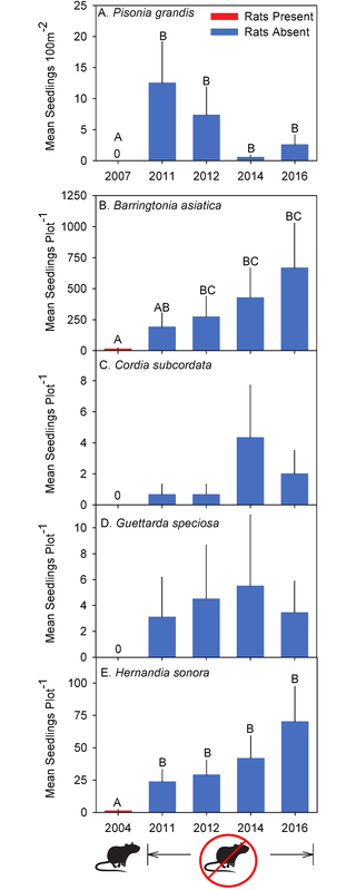
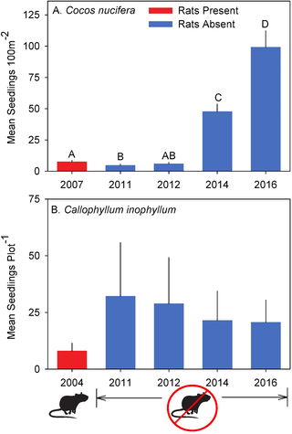
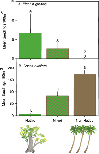
Here are some figures that we got from the original research paper (where we got the data from). Later, you’ll replicate them and you can decide who’s you like more!
Function Fun 2: Agregating and Plotting
Agregating Functions
tree_type_table
This function takes in a DataFrame and a string, and does all of the following, each on one line:
Filter for only rows where the column
Treehas the valuenameGroup the data by what year it was collected
Sum the total count in each row for the year
Return the table with it’s original index
def tree_type_table(table: pd.DataFrame, name: str):
    tree = (table.query(f"Tree == '{name}'")
              .groupby("Year")
              .agg({"Count": "sum", "Rats":first})
              .reset_index())
    return tree
triple_seedling_table
This function is a bit more complicated, so we’ll go though it quickly; if you’re interested, you’re more than welcome to try to figure it out, but it is more advanced than the majority of this notebook.
triple_seedlings_table does the following:
creates a table
mainwhich selects relevant columnscreates a table
forestwhich ismain, but only in the year 2016creates a table
ratswhich ismainwhich performs a similar aggregation totree_type_tableas the name suggests, the function returns all 3 tables
def triple_seedling_table(table: pd.DataFrame, genus: str):
    main = (table[[f'{genus} Count','Year', 'Forest', 'Rats']]
                     .rename(columns = {f'{genus} Count': "Count"}))

    forest = (main.drop(columns="Rats")
                   .query("Year == 2016"))

    rats = (main.drop(columns="Forest")
                .groupby("Year")
                .agg({"Count": "sum", "Rats": first})
                .reset_index())
    return main, forest, rats
Plotting Functions
plot_rats
You don’t need to worry about the implementation of this function, but it will give you a nicely formatted graph given a Table/DataFrame. This function should ideally have one column named 'Year', one named 'Count', and one named 'Rats'. If it has these three functions you can simply call the following:
plot_rats(data_frame)If your data frame doesn’t have all of these, you’ll need to call the function as so:
plot_rats(data = data_frame, x = x axis, y = y axis, color = group column)where all of the values right of the = are filled in by you. You may also optionally include the argument:
title = "Your Title"
The implementation of the function can be found below, and if you’re interested, you can read the documentation of the pandas and plotly modules which make this function work.
def plot_rats(data, x = None, y = None, color = None, title = None):
    cols = pd.Series(['Year', 'Count', 'Rats'])
    present = cols.isin(data.columns).all()
    if present:
        fig = px.bar(data_frame = data, x='Year', y="Count", color = 'Rats',
                       color_discrete_sequence =['#a63932', '#003262'],
                       title = title) #, width = 1000, height = 500)
    else:
        fig = px.bar(data_frame = data, x=x, y=y, color = color,
                       color_discrete_sequence =['#a63932', '#003262'],
                       title = title) #, width = 1000, height = 500)
    fig.update_xaxes(type = 'category')
    fig.show()
plot_forest
This function functions in a very similar fashion. It takes in a dataframe, and outputs an interactive bar graph!
def plot_forest(df, title = None):
    grouped = df.groupby(["Year", "Forest"]).sum().reset_index().drop(columns="Year")
    plot = px.bar(data_frame = grouped, x = "Forest", y = "Count", color = "Forest",
      color_discrete_sequence = ["#823e2b",'#85683c', "#3e853c"], title = title) #, width = 1000, height = 500
    plot.show()
Results
The long awaited end has arrived! Theres no more work for you to do in this section. Simply run the cell below to see what all of your hard work has created. Go you!
Agregating Results
Play Around a bit with the cell below after running it to view the tables you just made!
@interact(Function = widgets.Dropdown(options = ["tree_type", "seedlings"]))
def the_tables(Function):
    if Function == "tree_type":
        @interact(Tree = widgets.Dropdown(options = ['Barr', 'Calo', 'Cord', 'Guet', 'Hern']))
        def show_me_tree_type(Tree):
            tree_type_table(trees, Tree).show()
    else:
        @interact(Tree = widgets.Dropdown(options = ['Pisona', "Coco"]),
                  Rows = widgets.BoundedIntText(value = 10, max = 30, min = 1))
        def show_me_seedlings(Tree, Rows):
            a, b, c = triple_seedling_table(seedlings, Tree)
            for df in [a, b]:
                df.show(rows = Rows)
Aggregate the Tables
This cell is just nicely formatted and supplies all the tables from the data, using only your functions!
(barrs, calos, cords, guets, herns,
(pisonia, pisona_forest, pisona_rats),
(coco, coco_forest, coco_rats))          = (tree_type_table(trees, 'Barr'),
                                            tree_type_table(trees, 'Calo'),
                                            tree_type_table(trees, 'Cord'),
                                            tree_type_table(trees, 'Guet'),
                                            tree_type_table(trees, 'Hern'),
                                            triple_seedling_table(seedlings, "Pisona"),
                                            triple_seedling_table(seedlings, "Coco"))
tree_dict = {"Plot Forests": {"Pisona": pisona_forest, "Coco": coco_forest},
             "Plot Rats": {"Barr": barrs, "Calo": calos, "Cord": cords, "Guet": guets, "Hern": herns, "Pisona": pisona_rats, "Coco": coco_rats}}
Plotting Results
Use the cell below to view some of the graphs you just made!
@interact(show_all = widgets.ToggleButton(value=False, description='Show All Tables', icon = "eye", button_style = "success"),
          Function = widgets.Dropdown(options = ["Plot Forests", "Plot Rats"]))
def the_plots(show_all, Function):
    if show_all:
        frst_lbl, sdlgs_lbl  = iter(['Cocos', "Pisonas"]), iter(["Barrs", "Calos", "Cords", "Guets", "Herns", "Pisonas", "Cocos"])
        for data in (coco_forest, pisona_forest):
            plot_forest(data, title = next(frst_lbl))
        for data in (barrs, calos, cords, guets, herns, pisona_rats, coco_rats):
            plot_rats(data, title = next(sdlgs_lbl))
    elif Function == "Plot Rats":
        @interact(Tree = widgets.Dropdown(options = ['Barr', 'Calo', 'Cord', 'Guet', 'Hern']))
        def show_me_rats(Tree):
            plot_rats(tree_dict[Function][Tree], title = Tree)
    else:
        @interact(Tree = widgets.Dropdown(options = ['Pisona', "Coco"]))
        def show_me_forest(Tree):
            plot_forest(tree_dict[Function][Tree], title = Tree)