# Initialize Otter
import otter
grader = otter.Notebook("engin-7-numerical.ipynb")

Numerical Integration and Differentiation¶

You must submit the lab to Gradescope by the due date. You will submit the zip file produced by running the final cell of the assignment.

About this Lab¶

The objective of this assignment is to familiarize you with numerical differentiation and integration.

Auto-grader¶

You will be provided with some test cases (i.e., sample input data) and associated answers (i.e., expected outputs) that you can use to help check your code. The provided test cases are not exhaustive, and it is your responsibility to ensure that your code works in general, not just for a few supplied test cases. We may use additional hidden test cases in grading your lab assignments.

Run the first cell, Initialize Otter, to import the auto-grader and submission exporter.

Answer cells¶

Throughout the assignment, replace ... with your answers. We use ... as a placeholder and these should be deleted and replaced with your answers.

Your answers must be in the cells marked # ANSWER CELL, including your final calculation/code. However, do not perform scratch-work in # ANSWER CELL. Add a new cell to perform your scratch-work. Your scratch-work will not be graded and does not need to be included in your submission unless otherwise noted.

To read the documentation on a Python function, you can type help() and add the function name between parentheses.

Score Breakdown¶

Question	Points
1	10.0
2	7.0
3	8.0
Total	25.0

Run the cell below, to import the required modules.

# Please run this cell, and do not modify the contents
import numpy as np
import math
import matplotlib.pyplot as plt
import scipy
from scipy.optimize import fsolve
np.seterr(all='ignore');

import hashlib
def get_hash(num):
    """Helper function for assessing correctness"""
    return hashlib.md5(str(num).encode()).hexdigest()

Question 1: Helicopter Speed Check¶

A helicopter pilot is flying above a road and monitors the cars traveling below. The pilot records the positions of the cars at regular intervals. The speed and acceleration can then be computed using finite difference formulas. Recall the approximations we discussed in lecture for an evenly spaced grid where $x_{j+1}-x_{j} = h$ for all $j$ :

Forward Difference
$\frac{df}{dx}\Big\rvert_{x_j} \approx \frac{f(x_{j+1})-f(x_j)}{h}$
(1)
Backward Difference
$\frac{df}{dx}\Big\rvert_{x_j} \approx \frac{f(x_{j})-f(x_{j-1})}{h}$
(2)
Central Difference
$\frac{df}{dx}\Big\rvert_{x_j} \approx \frac{f(x_{j+1})-f(x_{j-1})}{2h}$
(3)
Second-order Central Difference
$\frac{d^2f}{dx^2}\Big\rvert_{x_j} \approx \frac{f(x_{j+1})-2f(x_j)+f(x_{j-1})}{h^2}$
(4)

A visual representation of these derivative approximations is shown in Figure 1 below.

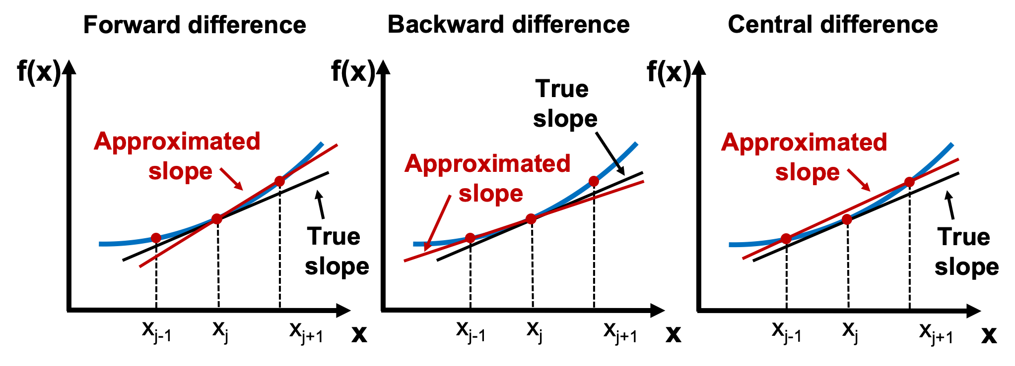
Figure 1. Finite difference methods.

Question 1.0: Forward Difference¶

Write a function forward_diff(x,t) where x and t are numpy arrays which contain the car coordinates and measurement times, respectively, i.e. the car was in position x[i] at time t[i]. You may assume that the time measurements in t are evenly spaced. The function should compute the velocity of the car using the forward difference method at the points in t for which it can be applied. Your function should return numpy arrays of the velocity and the times in t where it was evaluated (in this order).

Once you are done, try out your new forward_diff(x,t) function for the example below and make sure it produces the correct output. Assign the result to q1_0.

Examples:

>>> x = np.linspace(0,10,8)**4/4
>>> t = np.linspace(0,42,8)
>>> forward_diff(x, t)
(array([1.73538803e-01, 2.60308205e+00, 1.12800222e+01, 3.03692906e+01,
        6.40358184e+01, 1.16444537e+02, 1.91760378e+02]),
 array([ 0.,  6., 12., 18., 24., 30., 36.]))

# ANSWER CELL
...

# TEST YOUR FUNCTION HERE
q1_0 = ...
q1_0

grader.check("q1.0")

Question 1.1: Backward Difference¶

Write a function backward_diff(x,t) where x and t are numpy arrays which contain the car coordinates and measurement times, respectively, i.e. the car was in position x[i] at time t[i]. You may assume that the time measurements in t are evenly spaced. The function should compute the velocity of the car using the forward difference method at the points in t for which it can be applied.The function should compute the velocity of the car using the backward difference method at the points in t for which it can be applied. Your function should return numpy arrays of the velocity and the times in t where it was evaluated (in this order).

Once you are done, try out your new backward_diff(x,t) function for the example below and make sure it produces the correct output. Assign the result to q1_1.

Examples:

>>> x = np.linspace(0,10,8)**4/4
>>> t = np.linspace(0,42,8)
>>> backward_diff(x, t)
(array([1.73538803e-01, 2.60308205e+00, 1.12800222e+01, 3.03692906e+01,
        6.40358184e+01, 1.16444537e+02, 1.91760378e+02]),
 array([ 6., 12., 18., 24., 30., 36., 42.]))

# ANSWER CELL
...

# TEST YOUR FUNCTION HERE
q1_1 = ...
q1_1

grader.check("q1.1")

Question 1.2: Central Difference¶

Write a function central_diff(x,t) where x and t are numpy arrays which contain the car coordinates and measurement times, respectively, i.e. the car was in position x[i] at time t[i]. You may assume that the time measurements in t are evenly spaced. The function should compute the velocity of the car using the central difference method at the points in t for which it can be applied. Your function should return numpy arrays of the velocity and the times in t where it was evaluated (in this order).

Once you are done, try out your new central_diff(x,t) function for the example below and make sure it produces the correct output. Assign the result to q1_2.

Examples:

>>> x = np.linspace(0,10,8)**4/4
>>> t = np.linspace(0,42,8)
>>> central_diff(x, t)
(array([  1.38831043,   6.94155213,  20.82465639,  47.20255449,
         90.2401777 , 154.10245731]),
 array([ 6., 12., 18., 24., 30., 36.]))

# ANSWER CELL
...

# TEST YOUR FUNCTION HERE
q1_2 = ...
q1_2

grader.check("q1.2")

Question 1.3: Higher Order Derivatives¶

Write a function named second_central_diff(x,t) where x and t are numpy arrays which contain the car coordinates and measurement times, respectively, i.e. the car was in position x[i] at time t[i]. You may assume that the time measurements in t are evenly spaced. The function should compute the acceleration of the car using the second-order central difference method at the points in t for which it can be applied. Your function should return numpy arrays of the acceleration and the times in t where it was evaluated (in this order).

Once you are done, try out your new second_central_diff(x,t) function for the example below and make sure it produces the correct output. Assign the result to q1_3.

Examples:

>>> x = np.linspace(0,10,8)**4/4
>>> t = np.linspace(0,42,8)
>>> second_central_diff(x,t)
(array([ 2.42954325,  8.67694016, 19.08926836, 33.66652784, 52.40871859,
        75.31584062]),
 array([ 6., 12., 18., 24., 30., 36.]))

# ANSWER CELL
...

# TEST YOUR FUNCTION HERE
q1_3 = ...
q1_3

grader.check("q1.3")

Question 1.4¶

Let us now plot the first derivative approximation and compare them.

Define a function plot_finite_difference(x,t) which returns a matplotlib.pyplot figure of the velocity computed using the three finite difference methods.

The function should create the figure as follows:

Line plot (1) time vs. velocity as computed by the forward difference method at the points where it is valid
Line plot (2) time vs. velocity as computed by the backward difference method at the points where it is valid
Line plot (3) time vs. velocity as computed by the central difference method at the points where it is valid
A legend with labels ‘Forward difference’,‘Backward difference’ and ‘Central difference’ for line plots 1,2 and 3, respectively
X axis label which reads ‘Time, s’
Y axis label which reads ‘Velocity, ft/s’
X-axis limits $[0,45]$
Y-axis limits $[0,200]$
Title label which reads ‘Finite difference approximations’

Once you are done, test your function for x = np.linspace(0,10,8)**4/4 and t = np.linspace(0,42,8). Assign the result to q1_4. Your output figure should look like Figure 2 shown below. Feel free to experiment with other inputs as well as any plotting options that are not explicitly specified.

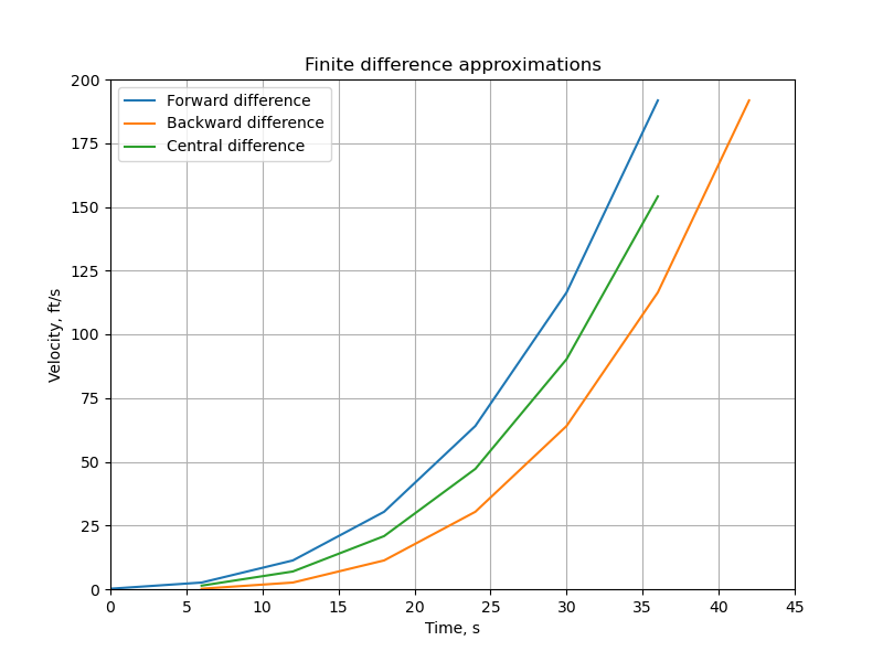
Figure 2. Finite difference approximations of the velocity.

# ANSWER CELL

# Do not modify this line
import matplotlib.pyplot as plt

...

# TEST YOUR FUNCTION HERE
q1_4 = ...

grader.check("q1.4")

Question 2: Gaussian Integral¶

In statistics, the normal or Gaussian distribution plays an important role and is widely used in the natural and social sciences. The density $f$ of the zero-mean, one-standard deviation Gaussian distribution (also known as the standard Gaussian distribution) shown in Figure 3 is given by:

f(x) = \frac{1}{\sqrt{2\pi}}e^{-\frac{-x^2}{2}}

(5)

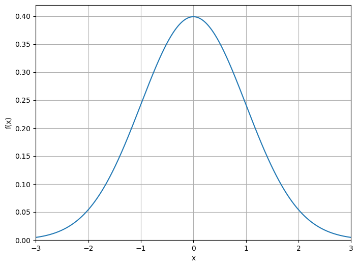
Figure 3: Standard Gaussian distribution

In many applications, such as computing the probability that $a < x < b$ , this function must be integrated as follows:

P(a < x < b)= I = \int^a_{b}{\frac{1}{\sqrt{2\pi}}e^{-\frac{x^2}{2}} dx}

(6)

However, this integral is impossible to solve analytically, necessitating the use of numerical integration.

In this problem, you’ll explore numerical integration methods to compute $I$ .

Question 2.0: Probability Density¶

Write a function prob_density(x) which computes and returns the value of the probability density $f(x)$ of the standard Gaussian distributon at each point in x. The output should be of the same type and size as x which may be a scalar float or a numpy.array of floats.

Once you are done, try out your new prob_density(x) function for the examples below and make sure it produces the correct output. Assign the result to q2_0.

Examples:

>>> prob_density(0.)
0.3989422804014327

>>>  prob_density(1.)
0.24197072451914337

>>> prob_density(np.linspace(-3,3,3))
array([0.00443185, 0.39894228, 0.00443185])

# ANSWER CELL
...

# TEST YOUR FUNCTION HERE
q2_0 = ...
q2_0

grader.check("q2.0")

Question 2.1: Left Riemann Integral¶

Write a function left_riemann(a,b,n) which approximates the integral $I$ where a, b are the constants described above and n is a positive integer representing the number of subintervals. Specifically, the interval $[a,b]$ should be divided into n equal parts such that the interval endpoints are $x_0, x_1, x_2, \dots, x_{n-1}, x_{n}$ . Your function should then numerically integrate $f(x)$ , the density function of the standard normal distribution, between $a$ and $b$ using the left Riemann integral method.

Once you are done, try out your new left_riemann(a,b,n) function for the example below and make sure it produces the correct output. Note that there could be some very minor differences from the results below depending on how you calculate the area. However, these differences should not be significant and should still pass the autograder. Assign the result to q2_1.

Examples:

>>> left_riemann(-1,1,4)
0.6725218292245875

>>> left_riemann(-1,1,16)
0.6820590314814196

>>> left_riemann(1,2,10)
0.14541584950162642

# ANSWER CELL
...

# TEST YOUR FUNCTION HERE
q2_1 = ...
q2_1

grader.check("q2.1")

Question 2.2: Right Riemann Integral¶

Write a function right_riemann(a,b,n) which approximates the integral $I$ where a, b are the constants described above and n is a positive integer representing the number of subintervals. Specifically, the interval $[a,b]$ should be divided into n equal parts , similar to the previous part. Your function should then numerically integrate $f(x)$ , the density function of the standard normal distribution, between $a$ and $b$ using the right Riemann integral method.

Once you are done, try out your new right_riemann(a,b,n) function for the example below and make sure it produces the correct output. Note that there could be some very minor differences from the results below depending on how you calculate the area. However, these differences should not be significant and should still pass the autograder. Assign the result to q2_2.

Examples:

>>> right_riemann(-1,1,4)
0.6725218292245875

>>> right_riemann(-1,1,16)
0.6820590314814196

>>> right_riemann(1,2,10)
0.1266178737010309

# ANSWER CELL
...

# TEST YOUR FUNCTION HERE
q2_2 = ...
q2_2

grader.check("q2.2")

Question 2.3: Midpoint Rule¶

Write a function midpoint(a,b,n) which approximates the integral $I$ where a, b are the constants described above and n is a positive integer representing the number of subintervals. Specifically, the interval $[a,b]$ should be divided into n equal parts, similar to the previous part. Your function should then numerically integrate $f(x)$ , the density function of the standard normal distribution, between $a$ and $b$ using the midpoint rule.

Once you are done, try out your new midpoint(a,b,n) function for the example below and make sure it produces the correct output. Note that there could be some very minor differences from the results below depending on how you calculate the area. However, these differences should not be significant and should still pass the autograder. Assign the result to q2_3.

Examples:

>>> midpoint(-1,1,4)
0.6878055489576537

>>> midpoint(-1,1,16)
0.6830048457095261

>>> midpoint(1,2,10)
0.13584922130730184

# ANSWER CELL
...

# TEST YOUR FUNCTION HERE
q2_3 = ...
q2_3

grader.check("q2.3")

Question 3: Corrugated Sheets¶

Corrugated roofing is produced by pressing a flat sheet of aluminum into a sheet whose cross section resembles the shape of a sine wave (see Figures 4 and 5).

Figure 4: Corrugated sheet

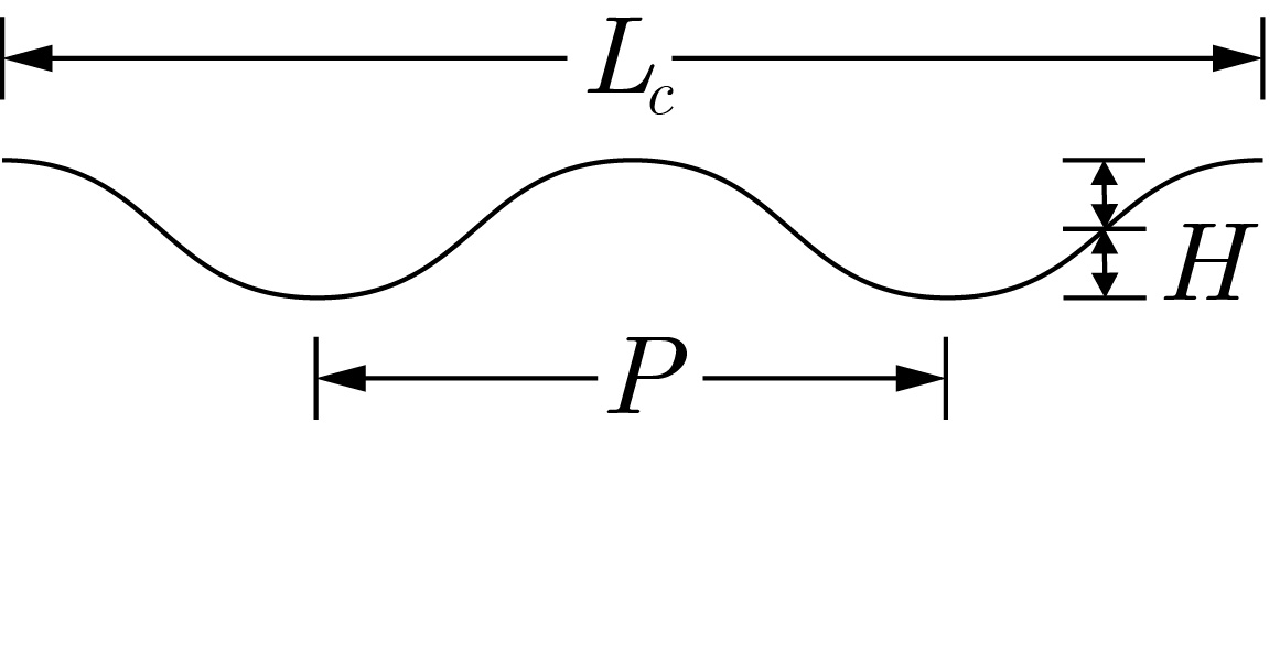
Figure 5: Corrugated sheet profile

Consider a corrugated sheet that is $L_C$ inches long, with a wave height of $H$ inches from the center line, and a wavelength of $P$ inches. To manufacture such a sheet, we need to determine the required length $L_F$ of the initial flat sheet. To compute $L_F$ , we determine the arc length of the wave, where the wave is given by $f(x) = H \sin\left(\dfrac{2\pi}{P} x\right)$ . Thus, we can compute the arc length $L_F$ using the equation

L_F = \int_0^{L_C}\sqrt{1+(f'(x))^2}dx

(7)

Where $f'(x)$ is given by:

f'(x) = \frac{2\pi H}{P}\cos\left(\frac{2\pi}{P}x\right)

(8)

In this problem, you’ll explore numerical integration methods to compute $L_F$ .

Question 3.0: Arc Length¶

Write a function arc_length(x,H,P) which computes and returns the value of the infinitesimal arc length $\sqrt{1+(f'(x))^2}$ , i.e. the integrand in the arc length function, for the given parameters H and P which are the wave height and wavelength, respectively (as given in the equations above). The output should be of the same type and size as x which may be a scalar float or a numpy.array of floats.

Once you are done, try out your new arc_length(x,H,P) function for the examples below and make sure it produces the correct output. Assign the result to q3_0.

Examples:

>>> arc_length(1.0,2,10)
1.42602888859332

>>>  arc_length(np.linspace(0,4,5),2,10)
array([1.60596909, 1.42602889, 1.07275073, 1.07275073, 1.42602889])

# ANSWER CELL
...

# TEST YOUR FUNCTION HERE
q3_0 = ...
q3_0

grader.check("q3.0")

Question 3.1: Trapezoid Rule¶

Write a function trapezoid(L_C,H,P,n) where n is the number of equal intervals, and L_C, H, and P are the corrugated length, wave height, and wavelength, respectively (as given in the equations above). Your function should compute an approximation of $L_F$ using the trapezoid rule.

Do not use any built-in integration functions.

Once you are done, try out your new trapezoid(L_C,H,P,n) function for the example below and make sure it produces the correct output. Note that there could be some very minor differences from the results below depending on how you calculate the area. However, these differences should not be significant and should still pass the autograder. Assign the result to q3_1.

Examples:

>>> trapezoid(72,1.5,2*np.pi,50)
102.89489835685144

>>> trapezoid(108,2,10,20)
140.68412785784827

 >>> trapezoid(90,2,8,30)
131.6522213593178

# ANSWER CELL
...

# TEST YOUR FUNCTION HERE
q3_1 = ...
q3_1

grader.check("q3.1")

Question 3.2: Simpson’s Rule¶

Write a function simpson(L_C,H,P,n) where n is the number of equal intervals, and L_C, H, and P are the corrugated length, wave height, and wavelength, respectively (as given in the equations above). Your function should compute an approximation of $L_F$ using Simpson’s rule.

Note that to use Simpson’s rule, you must have an odd number of grid points and, therefore, an even number of intervals. If the specified number of intervals n is odd, return the message “Number of intervals must be even.”

Do not use any built-in integration functions.

Once you are done, try out your new simpson(L_C,H,P,n) function for the example below and make sure it produces the correct output. Note that there could be some very minor differences from the results below depending on how you calculate the area. However, these differences should not be significant and should still pass the autograder. Assign the result to q3_2.

Examples:

>>> simpson(72,1.5,2*np.pi,50)
102.53506374537602

>>> simpson(108,2,10,20)
140.6332805053372

>>> simpson(90,2,8,30)
132.60485680897827

>>> simpson(90,2,8,31)
'Number of intervals must be even.'

# ANSWER CELL
...

# TEST YOUR FUNCTION HERE
q3_2 = ...
q3_2

grader.check("q3.1")

Question 3.3: Adaptive Quadrature¶

Write a function quad(L_C,H,P) where L_C, H, and P are the corrugated length, wave height, and wavelength, respectively (as given in the equations above). Your function should compute and return an approximation of $L_F$ using the built-in scipy.integrate.quad function which uses a more advanced method known as adaptive quadrature to compute integrals up to arbitrary precision. Refer to the documentation here. The required arguments are a function object which defines the function to be integrated as well as the lower and upper limits of integration. Note that scipy.integrate.quad will integrate the passed function along the axis corresponding to the first argument. If the function has additional arguments, as is the case with arc_length(x,H,P), they need to be passed to scipy.integrate.quad with the optional args argument. Use the default values for the remaining optional parameters. scipy.integrate.quad will return the value of the integral as well as an estimate of the absolute error.

Once you are done, try out your new quad(L_C,H,P) function for the example below and make sure it produces the correct output. Assign the result to q3_3.

Examples:

>>> quad(72,1.5,2*np.pi)
102.8880486715

>>> quad(108,2,10)
142.48321818018536

>>> quad(90,2,8)
131.73259251722146

# ANSWER CELL
...

# TEST YOUR FUNCTION HERE
q3_3 = ...
q3_3

grader.check("q3.3")

You’re done with this Lab!¶

Important submission information: After completing the assignment, click on the Save icon from the Tool Bar . After saving your notebook, run the cell with grader.check_all() and confirm that you pass the same tests as in the notebook. Then, run the final cell grader.export() and click the link to download the zip file. Then, go to Gradescope and submit the zip file to the corresponding assignment.

Once you have submitted, stay on the Gradescope page to confirm that you pass the same tests as in the notebook.

import matplotlib.image as mpimg
img = mpimg.imread('https://cal-icor.github.io/textbook.data/ucb/engin-7/animal.jpg')
imgplot = plt.imshow(img)
imgplot.axes.get_xaxis().set_visible(False)
imgplot.axes.get_yaxis().set_visible(False)
print("Congrats on finishing Lab 10!")
plt.show()

To double-check your work, the cell below will rerun all of the autograder tests.

grader.check_all()

Submission¶

Make sure you have run all cells in your notebook in order before running the cell below, so that all images/graphs appear in the output. The cell below will generate a zip file for you to submit. Please save before exporting!

Make sure you submit the .zip file to Gradescope.

# Save your notebook first, then run this cell to export your submission.
grader.export(pdf=False)