Estimated Time: 40 Minutes
Professor: Paul Li
Notebook Created By: Maria Sooklaris, Joshua Asuncion, Keilyn Yuzuki
Code Maintenance: Elias Saravia, Monica Wilkinson
Topics Covered
Welcome! This lab will be an introduction to Big Data and the Human Brain as well as a gentle introduction to Jupyter Notebooks. By the end of this lab you will be able to:
Define Big Data and dimensions in reference to a dataset.
Explain the high-level steps of simple computer facial recognition.
Identify reasons related to human cognition limits that we reduce the dimensions of big data during analysis.
Identify human ethics limitations/consequences that can result from reducing the dimensions of a large dataset.
Table of Contents
1. Jupyter Notebooks 
A Jupyter Notebook is an online, interactive computing environment, composed of different types of cells. Cells are chunks of code or text that are used to break up a larger notebook into smaller, more manageable parts and to let the viewer modify and interact with the elements of the notebook.
Notice that the notebook consists of 2 different kinds of cells: markdown and code. A markdown cell (like this one) contains text, while a code cell contains expressions in Python, the programming language in this Notebook.
1.1 Running Cells 
“Running” a cell is similar to pressing ‘Enter’ on a calculator once you’ve typed in an expression; it computes all of the expressions contained within the cell.
To run a code cell, you can do one of the following:
press Shift + Enter
click Cell -> Run Cells in the toolbar at the top of the screen.
You can navigate the cells by either clicking on them or by using your up and down arrow keys. Try running the cell below to see what happens.
print("Hello, World!")The input of the cell consists of the text/code that is contained within the cell’s enclosing box. Here, the input is an expression in Python that “prints” or repeats whatever text or number is passed in.
The output of running a cell is shown in the line immediately after it. Notice that markdown cells have no output.
2.1 What is Big Data? 
The term Big Data seems to be a buzz word everywhere lately, but what really is big data? Big data refers to an extremely large dataset that can be analyzed to reveal patterns, trends, or associations, especially relating to human behavior. Many companies and organizations collect data on every transaction or interaction of each user or consumer, so the data can grow very quickly!
Consider the image data that your brain deals with. From our eyes, we are constantly processing information which grows with every passing second. This adds up to a lot of data to process. Both computer programs and our brains deal with large amounts of data every day and we have developed strategies of efficiently processing this information.
2.2 Dimensionality 
Dimensionality refers to the size of the dataset (how many features or variables a dataset has). For example, if Berkeley had a dataset of students with each row, or observation, representing a student, some variables might be: year, major, residency, units, gpa, etc. A high dimensional dataset means that the number of features is very large and can exceed the number of observations, and calculations can become difficult.
3. Computer Vision: Recognizing Faces In An Image 
3.1 Overview of Facial Recognition 
Facial recognition systems are computer programs that analyze images of human faces in order to identify the individuals present in them. These systems have been used for situations such as general surveillance and personal security purposes (e.g. unlocking a smartphone). In general, these systems work by comparing selected facial features from a given image to faces that are already known within a database.
3.2 Ethics of Facial Recognition 
It is important to recognize that these systems are not always correct and the mistakes they make can be devastating to certain groups. Two well publicized controversies include Hewlett-Packard’s face-tracking web camera and Google’s facial recognition software in Google Photos. Desi Cryer, an African American man, uploaded a video in 2009 to YouTube showing that the HP face-tracking web camera did not track his face, while it had no problems tracking his white colleague. In a separate instance, Google’s Photos application labeled some African American people as “gorillas.” You can read more about the Google incident here.
Part of the problem with these facial recognition systems is that the data they use to train their algorithms is not representative of the entire population. A common training dataset is more than 75% male and more than 80% white, which could result in an algorithm incorrectly classifying minorities.
3.3 How Do These Systems Work? 
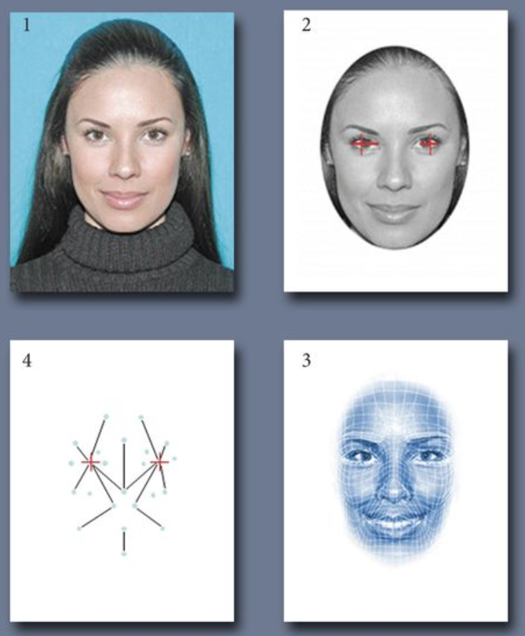
Facial recognition systems use computer algorithms to pick out distinctive features and details of a person’s face. The computer looks for ways that faces can be different, such as the distance between eyes, shading on the face, and many other features. Below are the steps of how common algorithms work:
Image is captured
Eye locations are determined
Image is converted to grayscale and cropped
Image is converted to a template used by the program for facial comparison results
Image is searched and matched using an algorithm to compare the template to other templates on file
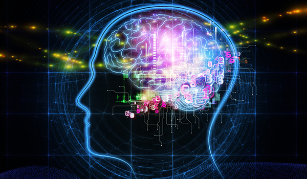
3.4 How Do Humans Recognize Faces? 
In early face recognition processing, the occipital lobe recognizes individual components of a face (e.g. eyes, ears, nose, etc.). Then, the fusiform gyrus, which is responsible for holistic information, is activated and combines the information together for further processing. This face is then compared to previous faces stored in your memory in order to recognize it. Humans recognize faces as a “sum of parts,” meaning that they recognize the face as a whole. In contrast, a computer recognizes the individual features of a face, and then if enough of these features are matched in its database, it determines the corresponding face.
4. Dimentionality Reduction 
4.1 The Data 
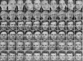
We will be using the Olivetti faces dataset, which contains a set of face images that were captured between April 1992 and April 1994 at AT&T Laboratories Cambridge. There are 10 different images of 40 distinct subjects. All of the images were taken against a dark background with the subjects facing the camera, but subjects were free to use different facial expressions. It is important to note that no efforts were made to create a diversified, unbiased population sample, and the participants were not chosen randomly. The images in this dataset do not represent the wider population of the US at the time, so any algorithm that was fed this data cannot be extrapolated to the rest of the country. Some example pictures are in the cell below. Check out this link for more information!
Before we being analyzing the data, we import Python packages that will help us visualize and understand the data. You do not need to know what the following code does. Run the cell below.
# Import packages that will be used later
import ipywidgets as widgets
from ipywidgets import interact, interact_manual
from IPython.display import display

from sklearn import decomposition
from sklearn.datasets import fetch_olivetti_faces

import numpy as np
import pandas as pd
import matplotlib.pyplot as plt

%matplotlib inline
Now, let’s load the data into the notebook. Again, you don’t have to know how the code is implemented, but think of it as “opening” the data like you would open an Excel file.
# Run to load the data
faces = fetch_olivetti_faces()
Given a dataset of facial images with a high number of dimensions, it can be very taxing for a computer to work with this data. Often, a process used to counter this issue is dimensionality reduction. When working with big data, we can perform an analysis where we look at the dimensions, or components, and order them in terms of their significance to the structure of the dataset. We can then reduce the number of dimensions by removing the least important components.
To see this in action, we can perform dimensionality reduction on the Olivetti faces dataset that we loaded. Run the code cell below to see what the face data actually looks like:
faces.datafaces.data.shapeWhen we talk about the faces data, each picture is actually represented as a sequence of a bunch of numbers. Each image is of size 64 x 64 pixels, and as a result the dimensionality is over 4,000. However, through this analysis we can easily reduce to 400 components and get approximations that are practically indistinguishable from the original images. We can reduce by even more and still get close approximations.
Run the following cell below. Try moving the slider representing the number of components to see how the accuracy changes. Look for when the faces become unrecognizable with their original images. To start, try to see what happens when we choose 50 components, 10 components and just 1 component. What do you see?
def dimensionality_reduction(x):
    pca = decomposition.PCA(n_components=x)
    pca.fit(faces.data)
    components = pca.transform(faces.data)
    projected = pca.inverse_transform(components)
    fig = plt.figure(figsize=(12, 10))
    for i in range(10):
        ax = fig.add_subplot(3, 5, i + 1, xticks=[], yticks=[])
        ax.imshow(projected[10*i].reshape(faces.images[10*i].shape), cmap=plt.cm.bone)

interact(dimensionality_reduction,
         x=widgets.IntSlider(min=1, max=400, step=1, value=200,
                             description='Number of Components:',
                             style={'description_width':'initial'},
                             layout=widgets.Layout(width='80%'),
                             continuous_update=False));
Discussion Question 1 (4 points): 
What do you notice about the faces as you change the number of principle components (2 pts)? What do the faces look like with 1 component (1 pt)? What about with more components (1 pt)?
WRITE YOUR ANSWER HERE. REPLACE THIS LINE WITH YOUR ANSWER BY DOUBLE-CLICKING THE CELL.
The process of dimensionality reduction is in fact finding the principal components of the data. The first few principal components are the most important components in determining the underlying structure of the data. In terms of a dataset containing images of faces, the first few components are the most important in determining the overall appearance of the face. They are associated with the lighting conditions of the face, while later components deal with certain features like eyes, noses, lips, etc.
Using this analysis, we can add and subtract different components until we get a good enough approximation of the data. By figuring out which components have the greatest importance, we are able to remove the less important components and in effect greatly reduce the size of the data we’re working with while maintaining a close resemblance to the original data.
5. Big Data Can Be Too Big! 
5.1 Why Would We Simplify Data? 
As we mentioned before, one of the reasons we would perform dimensionality reduction on big data is to speed up computation. Datasets can be trillions of rows big so any reduction or simplification of the data would positively affect processing and computing speed.
Another reason we would want to simplify data is to remove any noise from the dataset. Noise is essentially meaningless information contained within a dataset, such as corrupted or distorted data, often arrising from the data collection process. Ideally, we would want to remove any noisy data as it can negatively affect the results of any analysis.
Lastly, simplifying data allows us to make any analysis more likely to be understandable to humans. Especially in the context of machine learning, users that want to perform an analysis on big data with tools driven by machine learning might have a hard time understanding how a model works, and because of that they have a hard time controlling it and drawing any meaningful results. Simplifying the data and how to interact with the model helps users draw more meaningful results.
Abstracting away the low-level details of the user interface, or UI, of a model, is treating the model as a “black box.” Essentially, to simplify the data and the process, you create a mental model in which various inputs are put into the black box, which you assume works as it should, and the black box spits out various outputs. With this mental model, users only have to concern themselves with what they are inputting into the black box, and they don’t have to understand how exactly the machine learning process works. If you’re interested to learn more, check out this related article.
5.2 Risks With Simplifying Data 
When we alter any data into something other than its original form, we run the risk of affecting our analysis. We may inadvertantly introduce bias into the dataset while simplifying due to choosing to include, remove, combine, or alter certain aspects of the data. Depending on these assumptions, the analysis can be greatly affected, and conclusions may be compromised or incorrect.
Another potential risk is the risk of missing “edge cases” and its real-world implications. That is, if we simplify datasets to account for “most” variation, algorithms trained on that data can then fail to work well for edge cases. In real life, “edge cases” are often underrepresented minority groups in data. As previously mentioned, an example of this is facial recognition technology and the controversies with Google Images tagging dark-skinned people as “gorillas” and HP cameras only recognizing light-skinned faces.
5.3 Data Simplification Example 
Take the code cell below, for example. This shows the risks of simplifying data too much. If we take the example of life expectancy, we can predict how long a person would live based on other factors. Below, we show what happens if we train a model on all explanatory variables, versus just a single variable - and what could happen when attempting to reduce down data too much.
Run the cell below to start the widget. You can select from the list of variables either one or multiple variables to predict life expectancy. In order to select multiple, click and drag throught the list. You can also use the Command button and select features. This displays the accuracy of using the selected features to predict life expectancy, and plots the accuracy for each individual feature selected.
# just run this cell

from sklearn.model_selection import train_test_split
from sklearn.linear_model import LinearRegression

le = pd.read_csv('https://cal-icor.github.io/textbook.data/ucb/cogsci-1/life-expectancy.csv')
le = le.dropna()

train, test = train_test_split(le, test_size = 0.1, random_state = 42)
X_train = train.drop(['Country', 'Year', 'Status', 'Life expectancy '], axis = 1)
Y_train = train[['Life expectancy ']]

X_test = test.drop(['Country', 'Year', 'Status', 'Life expectancy '], axis = 1)
Y_test = test[['Life expectancy ']]

def predict_life_expectancy(variables):
    X_train = train[list(variables)]
    X_test = test[list(variables)]

    Y_train = train[['Life expectancy ']]
    Y_test = test[['Life expectancy ']]

    model = LinearRegression()
    model.fit(X_train, Y_train)

    print('Overall Model Accuracy: ', model.score(X_test, Y_test))

    plt.figure(figsize=(15,5))

    if len(variables) == 1:
        plt.bar(variables, model.score(X_test, Y_test))
        print('Model trained on: ', variables[0])
    if len(variables) > 1:
        print('Model trained on: ', variables)
        scores = []
        for v in list(variables):
            X_train = train[[v]]
            X_test = test[[v]]

            Y_train = train[['Life expectancy ']]
            Y_test = test[['Life expectancy ']]

            model = LinearRegression()
            model.fit(X_train, Y_train)
            scores.append(model.score(X_test, Y_test))

        plt.bar(list(variables), scores)
    plt.ylim(0, 1)
    plt.xlabel('Feature')
    plt.xticks(rotation=90)
    plt.ylabel('Single Feature Model Accuracy')
    plt.title('Life Expectancy Prediction Accuracy');

var = widgets.SelectMultiple(
    options=list(le.columns)[4:],
    value=['Adult Mortality'],
    rows=10,
    description='Variables',
    disabled=False
)

interact(predict_life_expectancy,  variables = var);
Discussion Question 2 (6 points): 
Which single feature gives you the best resulting accuracy (1 pt)? Worst accuracy (1 pt)? What combination of features results in the highest overall accuracy (2 pts)? What does this tell us about the risks of simplifying data (2 pts)?
WRITE YOUR ANSWER HERE. REPLACE THIS LINE WITH YOUR ANSWER BY DOUBLE-CLICKING THE CELL.
6. Conclusion 
In this lab you learned about Big Data and how prevalent it is in our daily lives. You saw how dimensions or features are used to measure the size of datasets, and how the size affects facial recognition in the interactive example. Then you explored the steps of computer facial recognition and the ways that humans reduce the dimensions of big data during analysis. You also learned about ethical limitations and consequences that can result from facial recognition as well as from simplifying data. These lessons and ideas can be applied to your later Cognitive Science coursework, and you can click on the links below to learn even more about these topics.
Please fill out this form to give us valuable feedback for later notebooks!
Submitting your work
Run the code cell below convert your answers to the discussion question into a pdf. Be sure to follow instructions for submitting this assignment.
After running the cell, you can click
Download it here!to create a PDF.After running the cell, you can also right-click on
Download it here!then clickSave Link As...to save it as a PDF.
# run this cell to convert your work to a pdf for submission
from otter import Notebook
Notebook.export("brain-vs-ml.ipynb", filter_type='tags')Additional Data Ethics Articles
Bibliography
Gael Varoquaux - Adapted example for “Dimensionality Reduction” section. https://
scipy -lectures .org /packages /scikit -learn /auto _examples /plot _eigenfaces .html Jake VanderPlas - Adapted example for “Dimensionality Reduction” section. notebooks
/05 .09 -Principal -Component -Analysis .ipynb Jupyter Widgets - Adapted code for widget. https://
ipywidgets .readthedocs .io /en /stable /index .html Raluca Budiu - Adapted article for “Why Would We Simplify Data?” section. https://
www .nngroup .com /articles /machine -learning -ux/ Scikit-learn - Used Olivetti Faces dataset. https://
scikit -learn .org /0 .19 /datasets /olivetti _faces .html Viatcheslav Wlassoff - Adapted article for “How Do Humans Recognize Faces?” section. https://
www .brainblogger .com /2015 /10 /17 /how -the -brain -recognizes -faces/
Data Science Opportunities
Notebook developed by: Maria Sooklaris, Joshua Asuncion, Keilyn Yuzuki, Elias Saravia, Monica Wilkinson
Data Science Modules: http://
Data Science Offerings at Berkeley: https://