Bivariate Regression

Professor: Jason Wittenberg
Authors: Eric Van Dusen, William McEachen

Table of Contents¶

Defining a Linear Model
Why OLS?
Formula for OLS
Defining line fitness

!pip install -U seaborn --quiet
import numpy as np
from scipy import stats
import pandas as pd
from ipywidgets import *
import seaborn as sns
import matplotlib.pyplot as plt
import statsmodels.formula.api as smf
from IPython.display import display, Markdown
%matplotlib inline

Linear Models:¶

When we have two continuous variables (one dependent, one independent), we can use bivariate regression to determine how closely the two are related. Biviarate regression is used to determine how changes in one variable -- the independent variable, often denoted $X$ -- can predict changes in another, the dependent variable, often denoted $y$ . Bivariate regression relies on a linear model, which follows the form $y= \alpha + \beta X$ , where $\alpha$ is the y-intercept and $\beta$ is the slope.

If we assume that the relationship between our variables is not perfect (or, in the real world, if there is some predictable inaccuracy in our measurement), we add an error term $\epsilon$ : $y= \alpha + \beta X + \epsilon$ .

Motivating Ordinary Least Squares¶

To understand how we might create an equation for two variables, let’s consider the relationship between GDP growth and incumbent vote share (from Lecture I). Let’s load in the data table where the GROWTH column represents GDP growth and the VOTE column represents incumbent vote share.

fair_df = pd.read_csv('https://cal-icor.github.io/textbook.data/ucb/pols-3/fair.csv')
fair_df

Now we can plot these variables: Review: Why is GDP growth our independent variable (represented on the x-axis)?

plot = sns.scatterplot(data=fair_df, x='GROWTH', y='VOTE', color='black')
plot.set_xlabel('GDP Growth per Capita')
plot.set_ylabel('Incumbent Vote Share')
plot;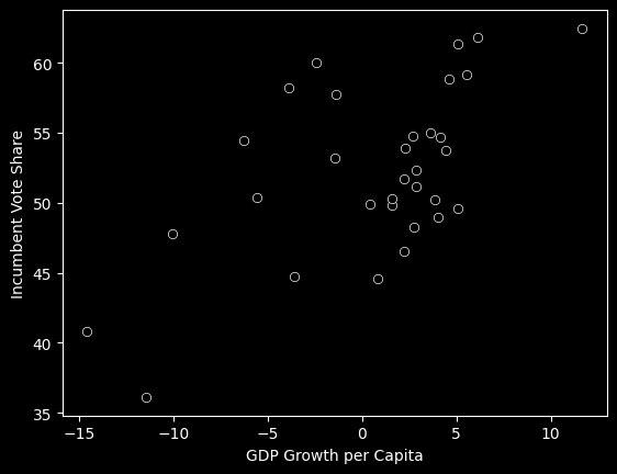

Above, it appears that as GROWTH increases (as we move further to the right on the x-axis), VOTE also increases. If we wanted to use this data to make future predictions, we could use a linear model to represent the variables’ relationship. Below, you can change the slope and intercept of the line to best fit the data:

def draw_line(slope, intercept):
    #The Linear Model
    def f(x):
        return intercept*(slope-1)/30*x +intercept
    x = np.arange(-15,15)
    y_pred = f(x)
    #The line
    plt.plot(x,y_pred)
    #The actual data
    sns.scatterplot(data=fair_df, x='GROWTH', y='VOTE', color='black')
    plt.xlabel('GDP Growth per Capita')
    plt.ylabel('Incumbent Vote Share')
    display(Markdown(rf'$\hat y$= {slope}$X$ + {intercept}:'))
    
interact(draw_line, slope=(0.0,3), intercept=(30,70));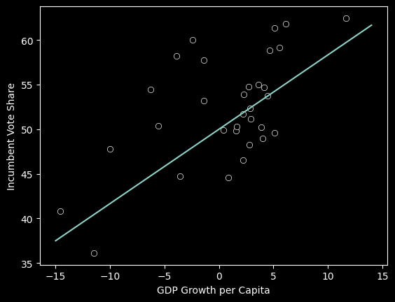

What line is best?¶

When we are evaulating how “good” a line is, we must address the residuals, the difference between the real and predicted values of y: $u_i = Y_i - \hat{Y_i}$ . Because every real y value has an associated residual, we need some way to aggregate the residuals if we are to measure the overall quality of a line

Absolute value¶

One measurement of loss is calculated by adding the absolute value of the residuals together:

\sum_{i=1}^n |u_i| = \sum_{i=1}^n |Y_i - \hat{Y_i}|

(1)

Squared error:¶

Another measurement is the squared error, calculated by adding the squared values of the residuals:

\sum_{i=1}^n |u_i^2| = \sum_{i=1}^n (Y_i-\hat{Y_i})^2

(2)

For either measurement, we want the line that results in the smallest value (indicating that the total difference between the predicted and actual values is small). Below, try to minimize either the absolute or squared loss:

def draw_line(slope, intercept):
    #The Linear Model
    def f(x):
        return intercept*(slope-1)/30*x +intercept
    x = np.arange(-15,15)
    y_pred = f(x)
    points = zip(fair_df.GROWTH, fair_df.VOTE)
    display(Markdown(rf'$\hat y$= {slope}$X$ + {intercept}:'))
    #The line
    plt.plot(x,y_pred)
    #The Data
    sns.scatterplot(data=fair_df, x='GROWTH', y='VOTE', color='black')
    plt.xlabel('GDP Growth per Capita')
    plt.ylabel('Incumbent Vote Share')
    #Print the loss
    print("Square Residual Sum:", sum([(y-f(x))**2 for x,y in points]))
    print("Absolute Residual Sum:", sum([abs(y-f(x))for x, y in points]))
    
interact(draw_line, slope=(0.0,3), intercept=(30,70), continuous_update=False);

What’s the smallest squared error/absolute error you can produce?

Ordinary Least Squares¶

Statisticians prefer to use the line that minimizes the squared residuals. To find the slope ( $\beta$ ) and y-intercept ( $\alpha$ ), the following equations are used:

\beta = \frac{\sum_{i=1}^n (X_i - \overline{X})(Y_i - \overline{Y})}{\sum_{i=1}^n (X_i - \overline{X})^2}

(3)

\alpha = \overline{Y}-\beta\overline{X}

(4)

Reminder: $\overline{X}$ represents the mean value of X.

Using Python:¶

To calculate the slope and y-intercept for the linear model of X and Y, use stats.linregress(X, Y). This returns a LinregressResult which holds the slope, intercept, the associated r and p values, and standard error (we’ll cover what those mean next). To access the slope and intercept, you can index into the LinregressResult, as shown below:

gdp_vote_result = stats.linregress(fair_df.GROWTH, fair_df.VOTE)
slope = gdp_vote_result[0]
intercept = gdp_vote_result[1]
slope, intercept

Now that we have the slope and intercept, we can plot the line of best fit alongside the original data:

sns.scatterplot(data=fair_df, x='GROWTH', y='VOTE', color='black')
plt.plot(fair_df.GROWTH, fair_df.GROWTH*slope +intercept, label='OLS model')
plt.xlabel('GDP Growth per Capita')
plt.ylabel('Incumbent Vote Share')
plt.legend()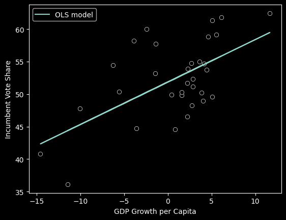

Goodness of Fit¶

Now that we have our linear model, we want to evaulate how well it tracks the relationship between the independent and dependent variables (X and Y). Below, which models are fit well by a linear model?

#A Generic Plotting function for some f(x)
def plot_func(f, label):
    x = np.random.randint(1,25, size=50)
    y = f(x)
    sns.scatterplot(x=x, y=y, label=label)
    result = stats.linregress(x, y)
    slope = result[0]
    intercept = result[1]
    plt.plot(x, x * slope + intercept, label='OLS model')
    plt.legend()

def f(x):
    return 2*x
plot_func(f, 'linear')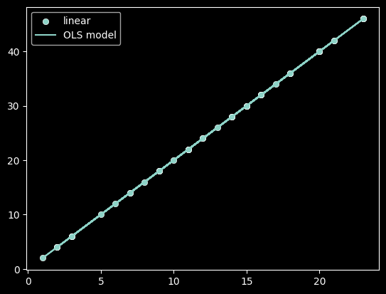

def f(x): 
    return 4*x**2 + np.random.random(50)
plot_func(f, 'quadratic')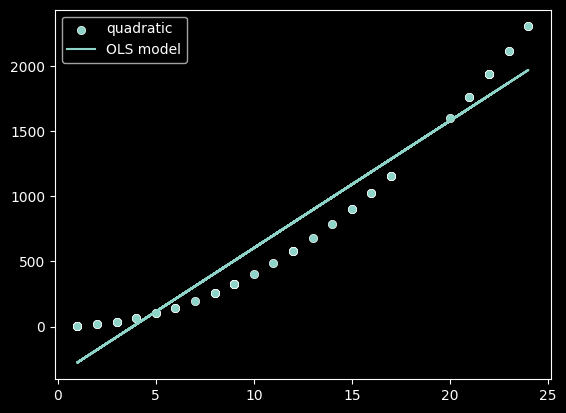

def f(x):
    return  8*np.log(x) + np.random.random(50)
plot_func(f, 'logarithmic')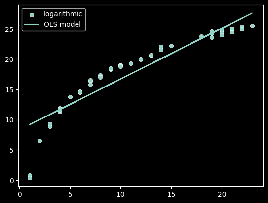

As we can see, linear models can better represent some relationships than others! We need some measure to quantify if a linear model is appropriate.

$R^2$ Statistic¶

In order to determine if our linear model is a good fit, we need to understand how much of the variance in the values of Y can be captured in our model. In the 3 plots above, a linear model had differing abilities to represent that variation.
Review: Which functions variation was best captured by a linear model?

We need a measurement that compares the overall variation in Y values with the variation that is not represented by our OLS model. This second kind is the residual variation because it is the difference between true values of Y and those predicted by our model. The $R^2$ statistic is a value between 0 and 1 that represents the proportion of variation in our Y value that can be accounted for by our model:

R^2 = 1-\frac{residual-variation}{total-variation}

(5)

The residual variation, or Residual Sum of Squares (RSS), is calculated by adding all squared residuals between the predicted and true values of Y:

RSS = \sum_{i=1}^n u_i^2 = \sum_{i=1}^n (Y_i - \hat{Y_i})^2

(6)

The total variation, or Total Sum of Squares (TSS), is calculated by adding the squared differences between each value of Y and the mean value of Y:

TSS = \sum_{i=1}^n (Y_i - \overline{Y})^2

(7)

Therefore, the $R^2$ statistic can be found thus:

R^2 = 1 - \frac{RSS}{TSS} = 1 - \frac{\sum_{i=1}^n (Y_i - \hat{Y_i})^2}{\sum_{i=1}^n (Y_i - \overline{Y})^2}

(8)

There is another formula for calculating $R^2$ using the Model Sum of Squares (MSS). The Model Sum of Squares is the total squared difference between predicted values of Y and the average value of Y:

MSS = \sum_{i=1}^n (\hat{Y_i} - \overline{Y})^2

(9)

The formula for $R^2$ using MSS is:

R^2 = \frac{MSS}{TSS} = \frac{\sum_{i=1}^n (\hat{Y_i}-\overline{Y})^2}{\sum_{i=1}^n (Y_i - \overline{Y})^2}

(10)

Using Python¶

There are 2 ways to calculate the $R^2$ value using Python. We will show both and demonstrate that they return the same result:

Write functions calculating the RSS and TSS, and then use those to calculate the $R^2$ statistic (we have done this below
Run stats.linregres(X, Y) and square the third value that it returns

#Method 1:
def rss(y, y_pred):
    """Return the Residual Sum of Squares between y and y_pred, the predicted values of y"""
    return sum((y - y_pred)**2)
def tss(y):
    """Return the Total Sum of Squares for y"""
    avg = np.mean(y)
    return sum((y - avg)**2)

def mss(y, y_pred):
    """Return the Model Sum of Squares for y and y_pred, the predicted values of y"""
    avg = np.mean(y)
    return sum((y_pred-avg)**2)

def r2(y, y_pred):
    """Return the R-squared statistic for y and the predicted values of y"""
    return 1 - (rss(y, y_pred) / tss(y))

predicted_y = fair_df.GROWTH*slope + intercept
r2(fair_df.VOTE, predicted_y)

#Method 2:
gdp_vote_result[2]**2

As we can see, the two results are the same! Why would this be the case?

Looking back to Lecture I, we recall that the correlation coefficient, r, is a function of the mutual variation for X and Y. While we can prove more rigorously that Pearson’s r is the square root of $R^2$ , that is outside the scope of this notebook. For a formal proof, follow this link.

Extrapolating to the Population¶

Once we have produced slope and intercept values for our model, we wish to know the potential applicability to the population at large. To do this, we return to the methods in Lecture I: finding variance and standard error values for the sample model.

To start, we must find the variance of residuals, or $\hat{\sigma}^2$ . This statistic is a measurement of the general difference between predicted and actual values of Y:

\hat{\sigma}^2 = \frac{\sum_{i=1}^n u_i^2}{n-2}

(11)

From the formula above, we can see that $\hat{\sigma}^2$ increases as the size of the residuals increase and decreases as our sample size, n, increases. We can then calculate the variance and standard error for the estimate of the slope value using the formula below:

var(\beta) = \frac{\hat{\sigma}^2}{\sum_{i=1}^n (X_i-\overline{X})^2}

(12)

se(\beta) = \sqrt{var(\beta)}

(13)

The Null Hypothesis¶

To calculate the t-statistic for a parameter (such as the slope of our model), we use the following formula:

t_\beta = \frac{\beta-\beta_0}{se(\beta)}

(14)

Above, $\beta_0$ is the value for our slope that we would expect under the null hypothesis.

Review: What is our null hypothesis for the value of the slope parameter?

Once we have calculated the t-statistic, we can use an online table (or in the appendix of your textbook) to find the p-value for whether there is a statistically significant relationship between X and Y.

Using Python¶

To find the p-value for the slope of our model, we use stats.linregress(X, Y). As we saw earlier, this returns the standard error as well, so we can find that using the same function. To access either value, index into the fourth value of the result for the p value, and the fifth value for the standard error.

gdp_vote_result = stats.linregress(fair_df.GROWTH, fair_df.VOTE)
gdp_vote_result

Interactive Visual¶

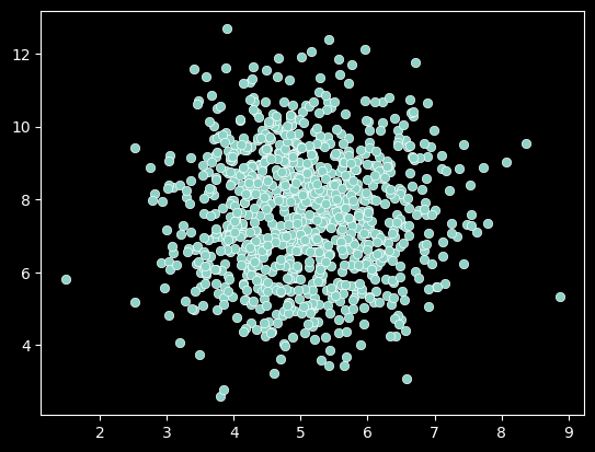
Below, we plot the relationship between two random variables. What happens to the results of the OLS model as you change the covariance? When you change the randomness of Y?

def cloud(covariance, rand_factor):
    X,Y = list(zip(*np.random.multivariate_normal([5,5], [[1,covariance],[covariance,1]], size=1000).tolist()))
    Y = Y+np.random.random(1000)*rand_factor
    sns.scatterplot(x=X, y=Y)
    print(stats.linregress(X,Y))
    print("R-value:",stats.pearsonr(X,Y)[0])

interact(cloud, covariance=(-1.0,1.0), rand_factor=(0,10), continuous_update=False);

Table of Contents¶

Linear Models:¶

Motivating Ordinary Least Squares¶

What line is best?¶

Absolute value¶

Squared error:¶

Ordinary Least Squares¶

Using Python:¶

Goodness of Fit¶

R2R^2R2 Statistic¶

Using Python¶

Extrapolating to the Population¶

The Null Hypothesis¶

Using Python¶

Interactive Visual¶

$R^2$ Statistic¶