Biodiversity

Run the cell below to setup the notebook (shift+return in cell to run or Press Run button in the menu) Do you see a number in the left margin of the cell below? If so, click on Kernel->Restart and Clear Output

%%capture
!pip install --no-cache-dir shapely
!pip install -U folium

%matplotlib inline
import os, time, folium, requests, json, random
import matplotlib.pyplot as plot, matplotlib as mpl
import numpy as np, pandas as pd
import ipywidgets as widgets

from matplotlib.collections import PatchCollection
from datetime import datetime
from shapely.geometry import Point, mapping
from shapely.geometry.polygon import Polygon

from datascience import *
from shapely import geometry as sg, wkt
from IPython.core.display import display, HTML

import httpimport
with httpimport.remote_repo(url='https://cal-icor.github.io/textbook.data/ucb/espm-105'):
    from espm_module import *

Natural History Museums and Data Science¶

The goal of this notebook is to demonstrate how to access and integrate diverse data sets to visualize correlations and patterns of species’ responses to environmental change. We will use programmatic tools (python) to show how to use Berkeley resources such as the biodiversity data from biocollections and online databases, field stations, climate models, and other environmental data. (Specifically we use data from the Berkeley Ecoengine, Cal-Adapt, and museum data via the GBIF API.)

Before we begin analyzing and visualizing biodiversity data, this introductory notebook will help familiarize you with the basics of programming in Python.

Table of Contents¶

0 - Jupyter Notebooks

1 - Python Basics

2 - GBIF API

3 - Comparing California Oak Species

4 - Cal-Adapt API

Part 0: Our Computing Environment, Jupyter notebooks ¶

This webpage is called a Jupyter notebook. A notebook is a place to write programs and view their results.

Text cells¶

In a notebook, each rectangle containing text or code is called a cell.

Text cells (like this one) can be edited by double-clicking on them. They’re written in a simple format called Markdown to add formatting and section headings. You don’t need to learn Markdown, but you might want to.

After you edit a text cell, click the “run cell” button at the top that looks like ▶| to confirm any changes. (Try not to delete the instructions of the lab.)

Code cells¶

Other cells contain code in the Python 3 language. Running a code cell will execute all of the code it contains.

To run the code in a code cell, first click on that cell to activate it. It’ll be highlighted with a little green or blue rectangle. Next, either press ▶| or hold down the shift key and press return or enter.

Try running this cell:

print("Hello, World!")

And this one:

print("\N{WAVING HAND SIGN}, \N{EARTH GLOBE ASIA-AUSTRALIA}!")
print("\N{grinning face}")

Part 1: Python basics ¶

Before getting into the more high level analyses we will do on the GBIF and Cal-Adapt data, we need to cover a few of the foundational elements of programming in Python.

A. Expressions¶

The departure point for all programming is the concept of the expression. An expression is a combination of variables, operators, and other Python elements that the language interprets and acts upon. Expressions act as a set of instructions to be fed through the interpreter, with the goal of generating specific outcomes. See below for some examples of basic expressions. Keep in mind that most of these just map to your understanding of mathematical expressions:

'you' + ' and me'

You will notice that only the last line in a cell gets printed out. If you want to see the values of previous expressions, you need to call the print function on that expression. Functions use parenthesis around their parameters, just like in math!

print(2 + 2)

print('you' + ' and I')

print(12 ** 2)

print(6 + 4)

B. Variables¶

In the example below, a and b are Python objects known as variables. We are giving an object (in this case, an integer and a float, two Python data types) a name that we can store for later use. To use that value, we can simply type the name that we stored the value as. Variables are stored within the notebook’s environment, meaning stored variable values carry over from cell to cell.

a = 4
b = 10/5

Notice that when you create a variable, unlike what you previously saw with the expressions, it does not print anything out.

We can continue to perform mathematical operations on these variables, which are now placeholders for what we’ve assigned:

print('a + b')

C. Lists¶

The following few cells will introduce the concept of lists.

A list is an ordered collection of objects. They allow us to store and access groups of variables and other objects for easy access and analysis. Check out this documentation for an in-depth look at the capabilities of lists.

To initialize a list, you use brackets. Putting objects separated by commas in between the brackets will add them to the list.

# an empty list
lst = []
print(lst)

# reassigning our empty list to a new list
lst = [1, 3, 6, 'lists', 'are' 'fun', 4]
print(lst)

To access a value in the list, put the index of the item you wish to access in brackets following the variable that stores the list. Lists in Python are zero-indexed, so the indicies for lst are 0, 1, 2, 3, 4, 5, and 6.

# Elements are selected like this:
example = lst[2]

# The above line selects the 3rd element of lst (list indices are 0-offset) and sets it to a variable named example.
print(example)

D. Dictonaries¶

Dictionaries are key-value pairs. Just like a word dictinary, you have a key that will index a specific definition.

my_dict = {'python': 'a large heavy-bodied nonvenomous constrictor snake occurring throughout the Old World tropics.'}

We can get a value back out by indexing the key:

my_dict['python']

But like real dictionaries, there can be more than one definition. You can keep a list, or even another dictionary within a specific key:

my_dict = {'python': ['a large heavy-bodied nonvenomous constrictor snake occurring throughout the Old World tropics.',
                      'a high-level general-purpose programming language.']}

We can index the list after the key:

my_dict['python'][0]

my_dict['python'][1]

Part 2: GBIF API¶

The Global Biodiversity Information Facility has an API or web service, which we can use to retrieve data. We will demonstrate several different species queries to the GBIF Web API.

You can think of a Web API as a fancy URL for machines; what do you think the end of this URL means?

http://api.gbif.org/v1/occurrence/search?year=1800,1899

If you guessed that it limits the search to the years 1800-1899, you’re right! Go ahead and click the URL above. You should see something like this:

{"offset":0,"limit":20,"endOfRecords":false,"count":5711947,"results":[{"key":14339704,"datasetKey":"857aa892-f762-11e1-a439-00145eb45e9a","publishingOrgKey":"6bcc0290-6e76-11db-bcd5-b8a03c50a862","publishingCountry":"FR","protocol":"BIOCASE","lastCrawled":"2013-09-07T07:06:34.000+0000","crawlId":1,"extensions":{},"basisOfRecord":"OBSERVATION","taxonKey":2809968,"kingdomKey":6,"phylumKey":7707728,"classKey":196,"orderKey":1169,"familyKey":7689,"genusKey":2849312,"speciesKey":2809968,"scientificName":"Orchis militaris L.","kingdom":"Plantae","phylum":"Tracheophyta","order":"Asparagales","family":"Orchidaceae","genus":"Orchis","species":"Orchis 

It might look like a mess, but it’s not! This is actually very structured data, and can easily be put into a table like format, though often programmers don’t do this because it’s just as easy to keep it as is. If you know the structure (thanks to the DarwinCore metadata standards), you can found what you’re interested in. Check out the api terms here: https://www.gbif.org/developer/occurrence#search

You might be able to pick out the curly braces { and think this it’s a dictionary. You’d be right, except in this format we call it JSON.

Aneides flavipunctatus, Black Salamander¶

When performing data analysis, it is always important to define a question that you seek the answer to. The goal of finding the answer to this question will ultimately drive the queries and analysis styles you choose to use/write.

For this example, we are going to ask: where have Aneides flavipunctatus (the Black Salamander) been documented? Are there records at any of our field stations?

The code to ask the API has already been written for us! This is often the case with programming, someone has already written the code, so we don’t have to. We’ll just set up the GBIFRequest object and assign that to the variable req, short for “request”:

req = GBIFRequest()  # creating a request to the API

Great, so how do we make searches? We can use a Python dictionary to create our query parameters. We’ll ask for the scientificName of the Black Salamander (Aneides flavipunctatus):

params = {'scientificName': 'Aneides flavipunctatus'}  # setting our parameters (the specific species we want)

Now that we have the parameters, we can feed this to our req variable to get back all the pages of data. We’ll then make sure that each record has a decimalLatitude, otherwise we’ll thow it out for now. Lastly, we’ll print out the first five records:

pages = req.get_pages(params)  # using those parameters to complete the request
records = [rec for page in pages for rec in page['results'] if rec.get('decimalLatitude')]  # sift out unmapped records
records[:5]  # print first 5 records

DataFrames¶

JSON is great, but it might be conceptually easier to make this a table. We’ll use the popular pandas Python library. In pandas, a DataFrame is a table that has several convenient features. For example, we can access the columns of the table like we would dictionaries, and we can also treat the columns and rows themselves as Python lists.

records_df = pd.DataFrame(records)   # converts the JSON above to a dataframe
records_df.head()  # prints the first five rows of the dataframe

Since each column (or row) above can be thought of as a list, that means we can use list functions to interact with them! One such function is the len function to get the number of elements in a list:

len(records_df.columns), len(records_df)

How many columns are there? (hint: first value) How many records/rows? (hint: it’s the other value)! That’s a lot of information. What variables do we have in the columns?

records_df.columns

We can use two methods from pandas to do a lot more. The value_counts() method will tabulate the frequency of the row value in a column, and the plot.barh() will plot us a horizontal bar chart:

records_df['country'].value_counts()

%matplotlib inline
records_df['country'].value_counts().plot.barh();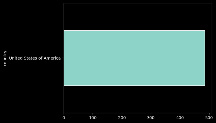

records_df['county'].value_counts().plot.barh(figsize=(18,10));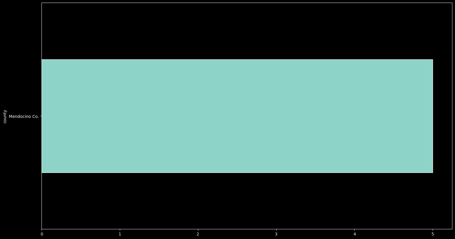

records_df['basisOfRecord'].value_counts().plot.barh();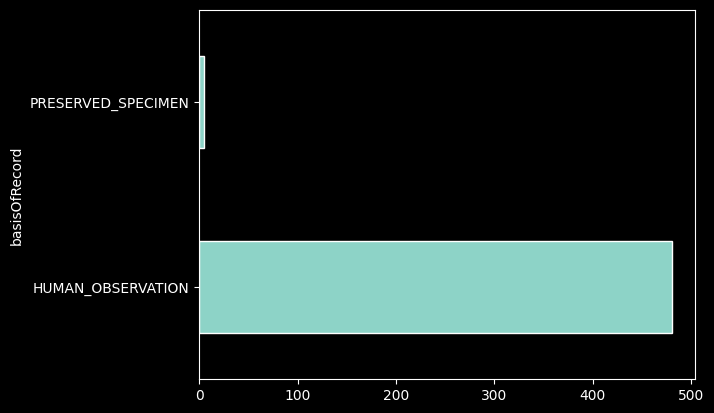

records_df['institutionCode'].value_counts().plot.barh();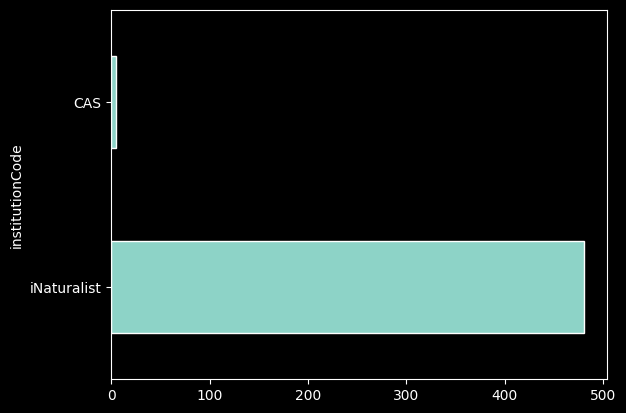

The groupby() method allows us to count based one column based on another, and then color the bar chart differently depending on a variable of our choice:

records_df.groupby(["institutionCode", "basisOfRecord"])['basisOfRecord'].count()

records_df.groupby(["institutionCode", "basisOfRecord"])['basisOfRecord'].count().unstack().plot.barh(stacked=True);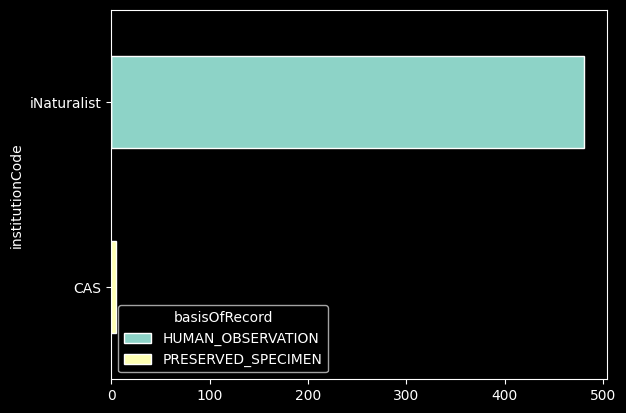

And we can use plot.hist() to make a histogram:

records_df['elevation'].plot.hist();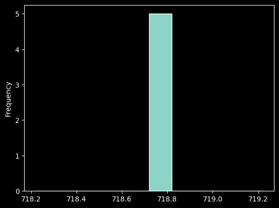

#When were these records collected?
records_df['year'].plot.hist();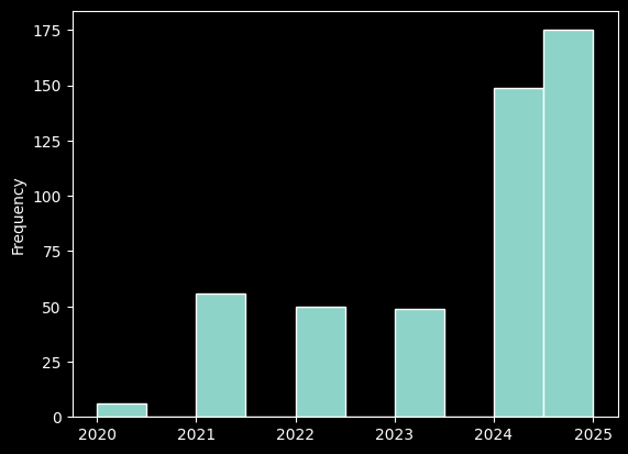

Mapping¶

Now we can map our latitude and longitude points. We’ll want to color code by institutionCode so we can see which collection made the observation or has the specimen. We’ll use a function that does this automatically, and it will randomly generate a color-- so if you don’t like the colors you see, try running the cell again!

color_dict, html_key = assign_colors(records_df, "institutionCode")
display(HTML(html_key))

#Did you get an error in the last cell? If so you may have a corrupt or old variable so please run this cell
#to re-run your original search
#If you did not get an error, skip this cell and keep going!

my_req = GBIFRequest()  # creating a request to the API
my_params = {'scientificName': 'Aneides flavipunctatus'}  # setting our parameters (the specific species we want)
my_pages = my_req.get_pages(my_params)  # using those parameters to complete the request
my_records = [rec for page in my_pages for rec in page['results'] if rec.get('decimalLatitude')]  # sift out valid records
records_df = pd.DataFrame(my_records) 

color_dict, html_key = assign_colors(records_df,'institutionCode');
display(HTML(html_key))

Now we can map the points!

mapa = folium.Map(location=[37.359276, -122.179626], zoom_start=5) # Folium is a useful library for generating
                                                                   # Google maps-like map visualizations.
for r in records_df.iterrows():
    lat = r[1]['decimalLatitude']
    long = r[1]['decimalLongitude']
    folium.CircleMarker((lat, long), color=color_dict[r[1]['institutionCode']], popup=r[1]['basisOfRecord']).add_to(mapa)
mapa

To get the boundries for all the reserves, we will need to send a request to get GeoJSON, which is a format for encoding a variety of geographic data structures. With this code, we can request GeoJSON for all reserves and plot ocurrences of the species. First we’ll assign the API URL that has the data to a new variable url:

url = 'https://ecoengine.berkeley.edu/api/layers/reserves/features/'

Now we make the requests just like we did earlier through the GBIF:

# NOTE: The following cell and any cells relying on the reserves variable will not work, as the EcoEngine API has been deprecated.
# A data request to the EcoEngine team is in progress to receive the data, and will be updated in the future.
# If this comment is still present, data has not yet been obtained; we recommend you skip to section 3.
reserves = requests.get(url, params={'page_size': 30}).json()
reserves

If you look closely, this is just bounding boxes for the latitude and longitude of the reserves.

There are some reserves that the EcoEngine didn’t catch, we’ll add the information for “Blodgett”, “Hopland”, and “Sagehen”:

station_urls = {
    'Blodgett': 'https://raw.githubusercontent.com/BNHM/spatial-layers/master/wkt/BlodgettForestResearchStation.wkt',
    'Hopland': 'https://raw.githubusercontent.com/BNHM/spatial-layers/master/wkt/HoplandResearchAndExtensionCenter.wkt',
    'Sagehen': 'https://raw.githubusercontent.com/BNHM/spatial-layers/master/wkt/SagehenCreekFieldStation.wkt'
}
reserves['features'] += [{'type': "Feature", 'properties': {"name": name}, 'geometry': mapping(wkt.loads(requests.get(url).text))}
                for name, url in station_urls.items()]

We can see all the station names by indexing the name value for the reserves:

[r['properties']['name'] for r in reserves['features']]

We can send this geojson directly to our mapping library folium. You’ll have to zoom in, but you should see blue outlines areas, there are the reserves!:

mapb = folium.Map(location=[37.359276, -122.179626], zoom_start=5) 

wkt = folium.features.GeoJson(reserves)
mapb.add_child(wkt)
for r in records_df.iterrows():
    lat = r[1]['decimalLatitude']
    long = r[1]['decimalLongitude']
    folium.CircleMarker((lat, long), color=color_dict[r[1]['institutionCode']], popup=r[1]['basisOfRecord']).add_to(mapb)
mapb

We can also find out which stations have how many our species. First we’ll have to add a column to our DataFrame that makes points out of the latitude and longitude coordinates:

def make_point(row):
    return Point(row['decimalLongitude'], row['decimalLatitude'])

records_df["point"] = records_df.apply(lambda row: make_point (row),axis=1)

Now we can write a little function to check whether that point is in one of the stations, and if it is, we’ll add that station in a new column called station:

def in_station(reserves, row):
    
    reserve_polygons = []

    for r in reserves['features']:
        name = r['properties']['name']
        poly = sg.shape(r['geometry'])
        reserve_polygons.append({"id": name,
                                 "geometry": poly})
    
    sid = False
    for r in reserve_polygons:
        if r['geometry'].contains(row['point']):
            sid = r['id']
            sid = r['id']
    if sid:
        return sid
    else:
        return False

Now apply this function to the DataFrame:

records_df["station"] = records_df.apply(lambda row: in_station(reserves, row),axis=1)
in_stations_df = records_df[records_df["station"] != False]
len(in_stations_df.columns), len(in_stations_df)

Let’s see if this corresponds to what we observed on the map:

in_stations_df.groupby(["species", "station"])['station'].count().unstack().plot.barh(stacked=True)

my_req = GBIFRequest()  # creating a request to the API
my_params = {'scientificName': 'Melanerpes formicivorus', 'basisOfRecord':'Preserved_Specimen'}  # search parameters (requesting a species and only Preserved specimens to filter out all the observations)
my_pages = my_req.get_pages(my_params)  # using those parameters to complete the request
my_records = [rec for page in my_pages for rec in page['results'] if rec.get('decimalLatitude')]  # sift out valid records
my_records_df = pd.DataFrame(my_records)  # make a dataframe
my_records_df.tail()  # print last 5 rows

len(my_records_df)

color_dict, html_key = assign_colors(my_records_df, "institutionCode")
display(HTML(html_key))

mapc = folium.Map([37.359276, -122.179626], zoom_start=5)

points = folium.features.GeoJson(reserves)
mapc.add_child(points)
for r in my_records_df.iterrows():
    lat = r[1]['decimalLatitude']
    long = r[1]['decimalLongitude']
    folium.CircleMarker((lat, long), color=color_dict[r[1]['institutionCode']]).add_to(mapc)
mapc

To see if your search results occur on a field station, run the following cells

def make_point(row):
    return Point(row['decimalLongitude'], row['decimalLatitude'])

my_records_df["point"] = my_records_df.apply(lambda row: make_point (row),axis=1)

my_records_df["station"] = my_records_df.apply(lambda row: in_station(reserves, row),axis=1)
in_stations_df = my_records_df[my_records_df["station"] != False]
len(in_stations_df.columns), len(in_stations_df)

How many records occur in field reserves according to the number of records above?

in_stations_df.groupby(["species", "station"])['station'].count().unstack().plot.barh(stacked=True)
in_stations_df.head()

Part 3: Comparing California Oak species:¶

Quercus douglassi	Quercus lobata	Quercus durata	Quercus agrifolia

California has high species diversity in its native oaks. Let’s search for these four species of oak using our GBIF API function and collect the observations:

species_records = []

species = ["Quercus douglasii", "Quercus lobata", "Quercus durata", "Quercus agrifolia"]

for s in species:
    req = GBIFRequest()  # creating a request to the API
    params = {'scientificName': s}  # setting our parameters (the specific species we want)
    pages = req.get_pages(params)  # using those parameters to complete the request
    records = [rec for page in pages for rec in page['results'] if rec.get('decimalLatitude')]  # sift out valid records
    species_records.extend(records)
    time.sleep(3)

We can convert this JSON to a DataFrame again:

records_df = pd.DataFrame(species_records)
records_df.head()

How many records do we have now?

len(records_df)

Let’s see how they’re distributed among our different species queries:

%matplotlib inline
records_df['scientificName'].value_counts().plot.barh()

We can group this again by collectionCode:

records_df.groupby(["scientificName", "collectionCode"])['collectionCode'].count().unstack().plot.barh(stacked=True)

We can also map these like we did with the first species search above:

color_dict, html_key = assign_colors(records_df, "species")
display(HTML(html_key))

mapc = folium.Map([37.359276, -122.179626], zoom_start=5)

points = folium.features.GeoJson(reserves)
mapc.add_child(points)
for r in records_df.iterrows():
    lat = r[1]['decimalLatitude']
    long = r[1]['decimalLongitude']
    folium.CircleMarker((lat, long), color=color_dict[r[1]['species']]).add_to(mapc)
mapc

We can use the same code we wrote earlier to see which reserves have which species of oak:

records_df["point"] = records_df.apply(lambda row: make_point (row),axis=1)
records_df["station"] = records_df.apply(lambda row: in_station(reserves, row),axis=1)
in_stations_df = records_df[records_df["station"] != False]
in_stations_df.head()

Now we can make a bar graph like we did before, grouping by species and stacking the bar based on station:

in_stations_df.groupby(["species", "station"])['station'].count().unstack().plot.barh(stacked=True)

---¶

Part 4: Cal-Adapt API¶

Let’s work with California Damsels dragonfly (Argia agrioides) data from the GBIF API and climate data from Cal-Adapt. (image from CalPhotos)

req = GBIFRequest()  # creating a request to the API
params = {'scientificName': 'Argia agrioides'}  # setting our parameters (the specific species we want)
pages = req.get_pages(params)  # using those parameters to complete the request
records = [rec for page in pages for rec in page['results'] if rec.get('decimalLatitude')]  # sift out valid records
records[:5]  # print first 5 records

We’ll make a DataFrame again for later use:

records_df = pd.DataFrame(records)
records_df.head()

Now we will use the Cal-Adapt web API to work with time series raster data. It will request an entire time series for any geometry and return a Pandas DataFrame object for each record in all of our Argia agrioides records:

req = CalAdaptRequest()
records_g = [dict(rec, geometry=sg.Point(rec['decimalLongitude'], rec['decimalLatitude']))
             for rec in records]
ca_df = req.concat_features(records_g, 'gbifID')

Let’s look at the first five rows:

ca_df.head()

len(ca_df.columns), len(ca_df)

This looks like the time series data we want for each record (the unique ID numbers as the columns). Each record has the projected temperature in Fahrenheit for 273 years (every row!). We can plot predictions for few random records:

# Make a line plot using the first 9 columns of dataframe
ca_df.iloc[:,:9].plot()

# Use matplotlib to title your plot.
plot.title('Argia agrioides - %s' % req.slug)

# Use matplotlib to add labels to the x and y axes of your plot.
plot.xlabel('Year', fontsize=18)
plot.ylabel('Degrees (Fahrenheit)', fontsize=16)

It looks like temperature is increasing across the board wherever these observations are occuring. We can calculate the average temperature for each year across observations in California:

tmax_means = ca_df.mean(axis=1)
tmax_means

What’s happening to the average temperature that Argia agrioides is going to experience in the coming years across California?

tmax_means.plot()

Is there a temperature at which the Argia agrioides cannot survive? Is there one in which they particularly thrive?

What if we look specifically at the field stations and reserves? We can grab our same code that checked whether a record was within a station, and then map those gbifIDs back to this temperature dataset:

records_df["point"] = records_df.apply(lambda row: make_point (row),axis=1)
records_df["station"] = records_df.apply(lambda row: in_station(reserves, row),axis=1)
in_stations_df = records_df[records_df["station"] != False]
in_stations_df[['gbifID', 'station']].head()

Recall the column headers of our ca_df are the gbifID:

ca_df.head()

Now we subset the temperature dataset for only the observations that occurr within the bounds of a reserve or field station:

station_obs = [str(id) for id in list(in_stations_df['gbifID'])]
ca_df[station_obs]

Let’s graph these observations from Santa Cruz Island against the average temperature across California where this species was observed:

plot.plot(tmax_means)
plot.plot(ca_df[station_obs])

# Use matplotlib to title your plot.
plot.title('Argia agrioides and temperatures in Santa Cruz Island')

# Use matplotlib to add labels to the x and y axes of your plot.
plot.xlabel('Year', fontsize=18)
plot.ylabel('Degrees (Fahrenheit)', fontsize=16)
plot.legend(["CA Average", "Santa Cruz Island"])

What does this tell you about Santa Cruz Island? As time goes on and the temperature increases, might Santa Cruz Island serve as a refuge for Argia agrioides?

To save a copy of your Jupyter Notebook with its output, use File-->Download as--> PDF as HTML (.PDF)